In one sentence: a virtual cell is a model that predicts how a cell’s state changes when we intervene. Foundation models learn the map; perturbation models learn the moves.
\[\text{new state} \;\sim\; f_\theta(\text{cell state},\ \text{intervention},\ \text{context})\]It is not a replacement for experiments, and it is not right just because it is big.
These are my notes after a long reading session on virtual cells. The video above (7:52) tells the story; this page keeps the same order, adds the tables I wanted while reading, and ends with a short script that reproduces the toy numbers. The tumor T-cell map, the 60/40 split, and the metric example are simulated for teaching; every other number comes from the papers listed at the end.
1. Why drug discovery wants a simulator
Of every ten drug candidates that enter human trials, about nine fail. Each approved drug costs about $2.6 billion (the Tufts estimate, which includes the cost of failures and of capital) and 10 to 15 years. The most common reason for failure is that the drug does not work in people: we bet on the wrong biology (my reading note on AI in drug discovery explains why Phase II is where the value hides).
Pilots train on simulators long before they fly a new plane. Biology has no such simulator, and the experimental space is far too large to test exhaustively:
| What you might test | Count |
|---|---|
| Single-gene knockouts | about 20,000 |
| Gene pairs | 199,990,000 |
| × cell types × doses × time points | many times more |
| Drug-like molecules | ~1060 (a common estimate) |
| The largest genome-wide CRISPR screen (Replogle et al., 2022) | > 2.5 million cells |
| Tahoe-100M drug atlas | ~100 million cells, 50 cancer lines, 379 drugs |
Even these heroic datasets cover only a small corner of the space. A model that could rank the untested experiments would be valuable.
2. Biology in 60 seconds: a cell is a state
Almost every cell in the body carries the same ~20,000 genes. A T cell differs from a neuron because it switches on different genes and copies them into RNA. Single-cell RNA sequencing (scRNA-seq) counts those RNA molecules, so each cell becomes a list of about 20,000 numbers: its state.
If you compress those lists onto a 2D map, similar cells land together (if PCA is new to you, see PCA explained with blood cells). In the running example, T cells from a tumor form three islands: fresh, fighting (effector), and exhausted. A drug or a gene edit is a perturbation: it pushes cells somewhere else on the map.
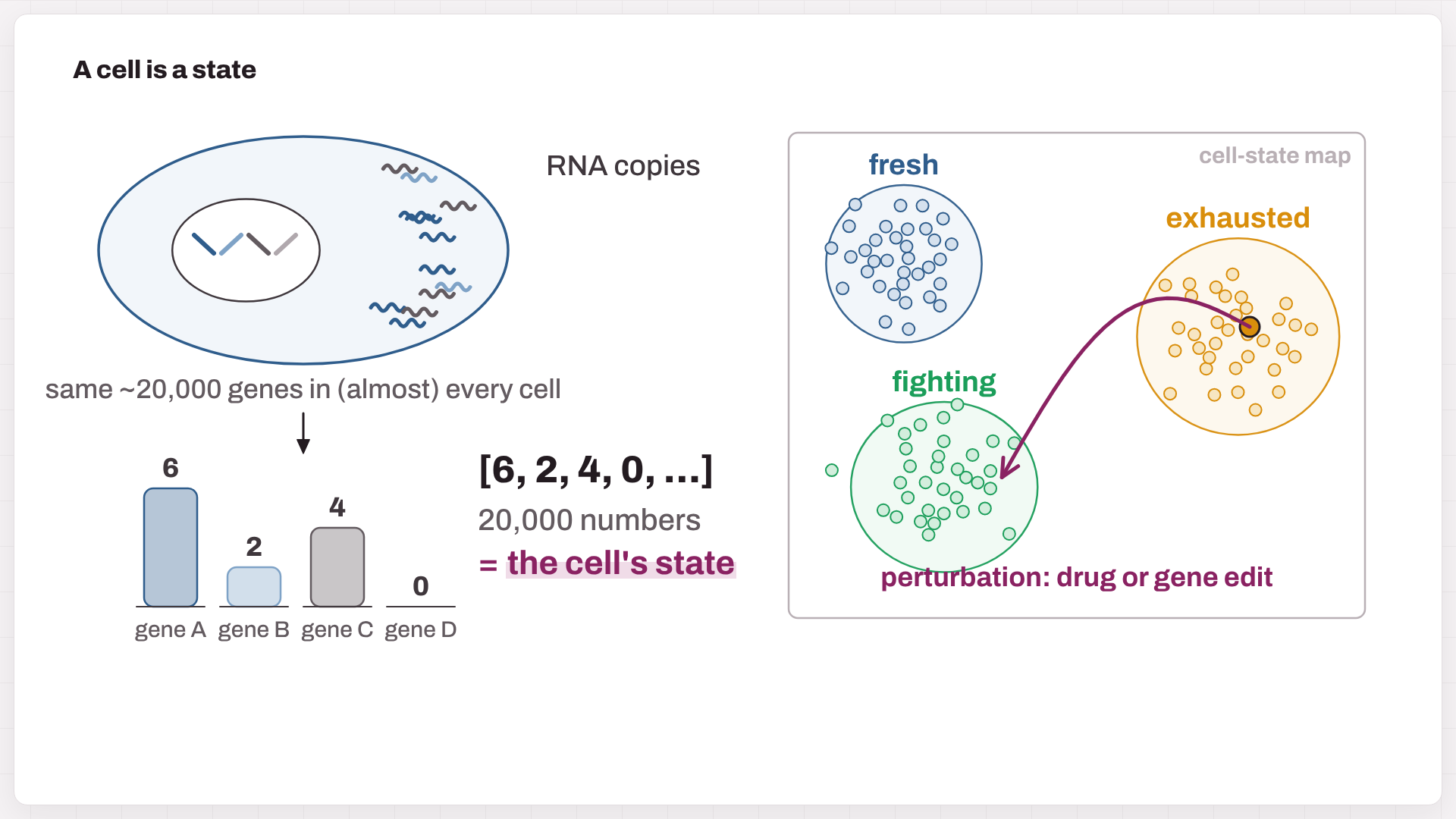
Fig. 1. RNA counts turn a cell into a vector of numbers, which becomes a point on a cell-state map. A perturbation is an arrow on that map.
3. What a virtual cell is
A virtual cell takes three inputs: a cell’s state, an intervention (a drug, a dose, a gene knockout), and the context (cell type, donor, time). It predicts the new state. Most designs share three steps (Ma et al., 2026):
- Encode the measured cell into a point on a learned map (an embedding).
- Transition: move the point according to the intervention and the context.
- Decode the moved point back into genes, or into another readout.
An older tradition simulates cells from equations; whole-cell models of the minimal bacterium JCVI-syn3A are a striking example. The new wave, laid out in the roadmap by Bunne et al. (Cell, 2024), learns these rules from millions of measured cells.
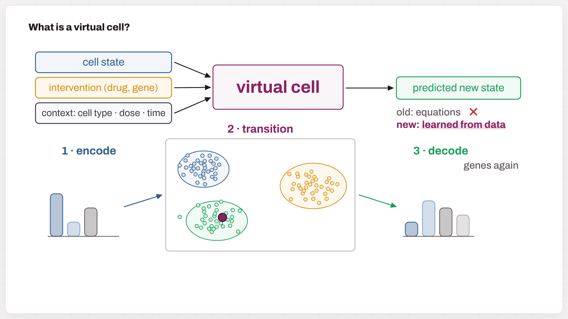
Fig. 2. A virtual cell maps (state, intervention, context) to a predicted new state. Most models can be read as encode → transition → decode.
4. Vocabulary in one table
| Term | One-line meaning | In cell models |
|---|---|---|
| Machine-learning model | a function with millions of adjustable knobs (parameters) | maps a cell profile to an output |
| Training | show examples, measure the error (the loss), and nudge the knobs to shrink it | e.g. predict held-out gene values |
| Deep learning | many layers stacked | transformers, graph networks, autoencoders |
| Transformer / attention | lets every token look at every other token (explainer) | every gene looks at every other gene |
| Self-supervised pretraining | fill in the blank; the data are their own answer key (how GPT is trained) | hide genes and guess them |
| Fine-tuning | a little more training on a small labelled task | cell-type labels, perturbation screens |
| Foundation model | pretrained once and reused for many tasks | Geneformer, scGPT, … |
| Embedding | a compact vector that summarizes a cell or a gene | the coordinates on the map |
| Perturbation · context | an intervention (knockout, CRISPRi, drug, dose) · where it applies (cell type, donor, time) | what the model is asked about |
| Unpaired data | control and treated cells are different cells | why models map clouds, not cells |
| Additive baseline | effect(A+B) ≈ effect(A) + effect(B) | the bar any pair predictor must clear |
5. Foundation models: learning the map
Treat each gene as a word and each cell as a sentence. During pretraining, the model hides some genes and guesses them from the rest. To fill the blank in Fig. 3, it has to notice PD-1, TIM-3 and LAG-3, infer an exhausted T cell, and guess TOX. Repeated over tens of millions of cells, this game teaches the “grammar” of co-expression.
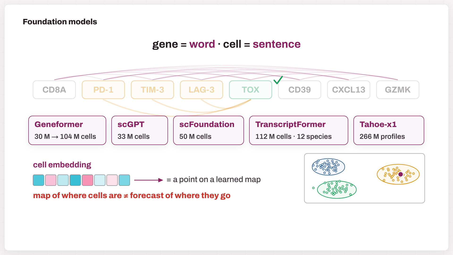
Fig. 3. Masked-gene pretraining, attention between genes, five well-known models, and the payoff: a cell embedding, which is a point on a learned map.
| Model | Input | Pretraining | Scale | Weights |
|---|---|---|---|---|
| Geneformer (Theodoris et al., Nature 2023) | genes ranked by expression | predict masked gene identities | 30 M → 104 M cells (V2) | open (Apache-2.0) |
| scGPT (Cui et al., Nat Methods 2024) | gene + expression-value tokens | predict expression from context | 33 M cells | code MIT; checkpoints public |
| scFoundation (Hao et al., Nat Methods 2024) | full profile + read depth | read-depth-aware reconstruction | 50 M cells, ~100 M parameters | non-commercial |
| TranscriptFormer (CZI, Science 2026) | genes + counts, protein-based gene vectors | generative, across 12 species | up to 112 M cells | open (MIT) |
| Tahoe-x1 (Tahoe, 2025 preprint) | expression profiles | masked expression, including drug-treated cells | 266 M profiles, up to 3 B parameters | open (Apache-2.0) |
The catch: a map of where cells are is not a forecast of where they go. A model can recognize your cells perfectly and still predict the wrong response to a knockout. Embeddings are also not automatically better than PCA on your own data; that has to be measured.
6. Perturbation models: learning the moves
Forecasts need experiments. Perturb-seq switches genes off with CRISPR and sequences every cell; drug screens (sci-Plex, Tahoe-100M) do the same with compounds. One fact shapes every model: sequencing destroys the cell, so we never see the same cell before and after. Models therefore learn to turn a cloud of control cells into a cloud of treated cells.
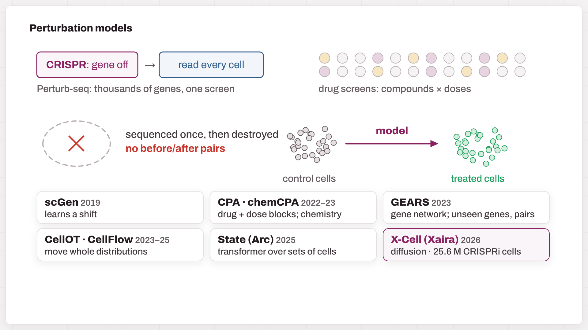
Fig. 4. CRISPR and drug screens supply the data. Because cells are destroyed when they are read, models map one population onto another. Six families of perturbation models.
| Model | Core idea | What it can extrapolate to |
|---|---|---|
| scGen (2019) | VAE; learn a treatment “shift” in latent space and apply it to other cells | a known treatment in a new cell type |
| CPA / chemCPA (2022–23) | add separate vectors for basal state, drug, dose and covariates; chemCPA encodes chemical structure | new doses and combinations; chemCPA: unseen compounds |
| GEARS (2023) | graph neural network over gene–gene relationships | unseen genes and gene pairs |
| CellOT / CellFlow (2023–25) | optimal transport / flow matching between whole distributions | heterogeneous responses, complex protocols |
| State (Arc, 2025–26) | transformer over sets of cells; trained on 167 M observational + > 100 M perturbed cells | responses across cell contexts |
| X-Cell (Xaira, 2026) | diffusion transformer over sets of cells, with biological priors | genetic perturbations in new contexts |
X-Cell, in more detail. X-Cell (Wang et al., 2026 bioRxiv) asks: given these cells’ current expression, what would they look like if we suppressed gene X? It takes control-cell profiles plus the identity of the target gene and returns predicted post-perturbation profiles for a population of cells. Three design choices stand out:
- It learns from real interventions. The X-Atlas/Pisces data hold about 25.6 million CRISPRi-perturbed cells from seven genome-scale screens. The paper counts 16 biological contexts, including cancer lines, iPSCs, resting and activated Jurkat cells, and differentiating iPSCs.
- It reads biological priors. Through cross-attention, it draws on representations of protein sequence, gene descriptions, interaction networks, genetic dependencies and cell morphology.
- It refines step by step. A masked diffusion process builds the predicted profile gradually, much as image generators do. “Diffusion” here describes the computation, not physical diffusion in the cell.
The authors report transfer to primary human CD4 T cells and to iPSC-derived melanocyte progenitors. That transfer includes self-supervised adaptation on control cells from the new context, so “zero-shot” still means some adaptation, just without perturbation data from that context. At the time of writing, the repository lists the weights and full inference code as “coming soon”, under a non-commercial CC BY-NC-SA 4.0 license. Treat it as a strong design to watch, pending independent replication.
Why predict distributions? In Fig. 5, a drug acts on 200 exhausted cells: 60% revive and 40% hold out. A model that predicts only the average lands between the two groups, where no real cell lives:
\[\mathbb{E}[\text{new state}] = 0.6\,\mu_{\text{revive}} + 0.4\,\mu_{\text{hold out}}\]The resistant subgroup is often exactly what a drug hunter needs to see.
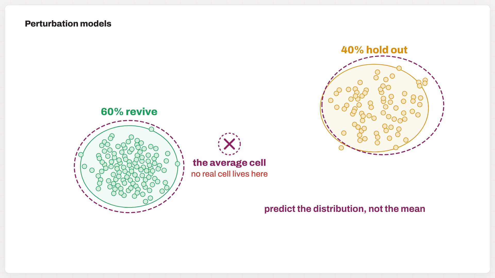
Fig. 5. Simulated: 60% of exhausted cells revive and 40% hold out. The mean prediction (×) lands where no cell lives; distribution models (dashed) keep both groups.
7. Where it helps in drug discovery
| Use | What the model does | Example |
|---|---|---|
| Targets | knock out every gene in silico; rank those that push diseased cells toward health | Geneformer nominated cardiomyopathy targets; CRISPR edits of top picks improved contraction of diseased iPSC heart cells (Theodoris et al., 2023) |
| Virtual screens | predict each compound’s transcriptional response; keep those that reverse the disease signature | chemCPA, Tahoe-x1-based response models |
| Combinations | rank which of ~200 M gene pairs (or drug pairs) deserve a real experiment | GEARS, CPA, CellFlow |
| Context and patients | carry responses over to new cell types and donors; flag responders and toxicity | State, X-Cell, CellFlow |
The model does not replace the lab. Its job is to narrow 20,000 options down to the 20 worth testing.
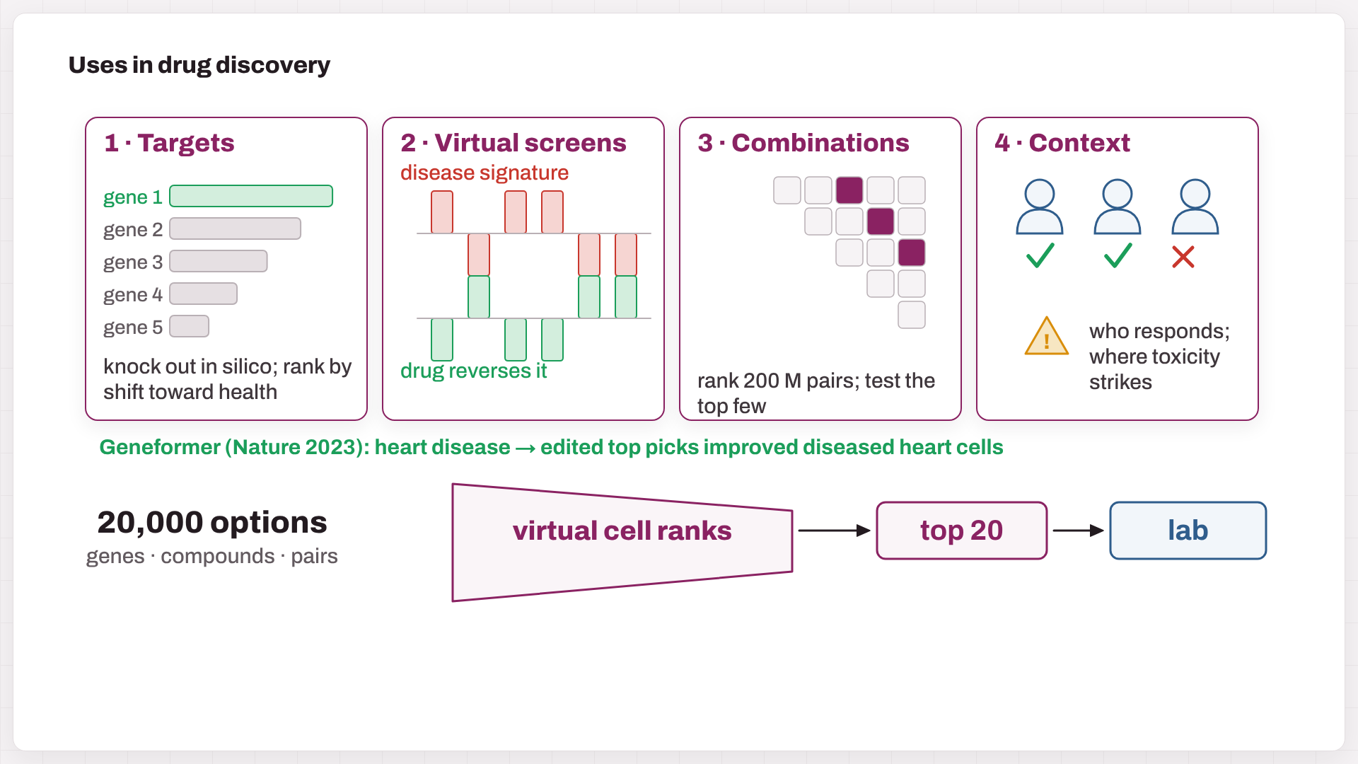
Fig. 6. Four uses, and the funnel that matters: 20,000 options → the virtual cell ranks them → the top 20 go to the lab.
8. Reality check: baselines and metrics
- Ahlmann-Eltze, Huber & Anders (Nature Methods, 2025) tested five foundation models and two other deep models. On gene pairs, none beat simply adding the two single-gene effects, and a linear model matched them on unseen single genes.
- Miller et al. (Nature Biotechnology, 2026) countered across 14 datasets: many common metrics are poorly calibrated, and with calibrated metrics, deep models do beat uninformative baselines.
- Arc’s Virtual Cell Challenge organizers reported the same tension: models were not yet consistently beating naive baselines across all metrics.
The toy example shows why metrics matter. Here 2,000 genes are measured and 60 truly change:
| Predictor | r (expression) | r (changes, Δ) |
|---|---|---|
| No change (copy the control) | 0.99 | n/a |
| Good model | 0.99 | 0.80 |
| Backwards (every change flipped) | 0.96 | −0.80 |
Correlation on raw expression is dominated by the 1,940 genes that do not move, so every predictor looks excellent. Score the changes and the truth appears.
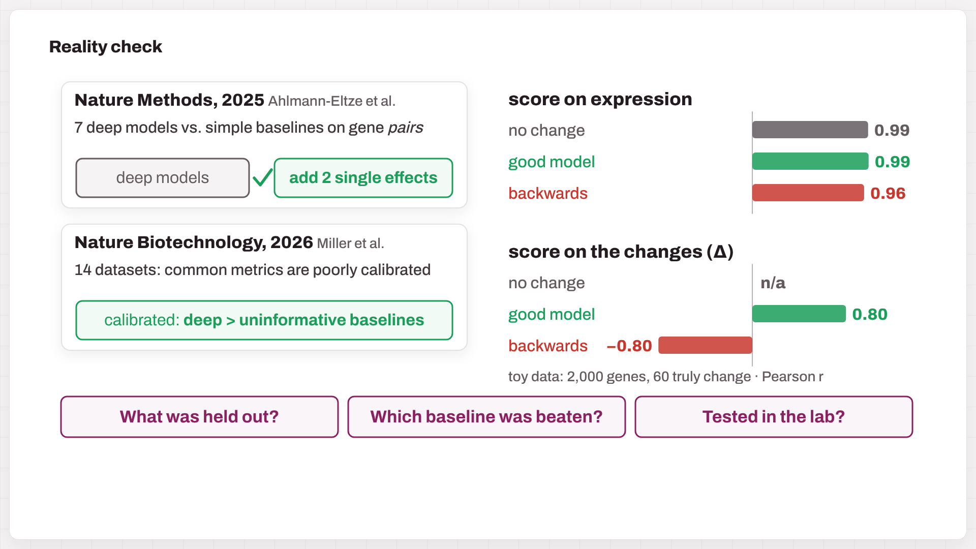
Fig. 7. Two benchmark papers, and the toy metric trap: scored on expression, a backwards model still reaches r = 0.96. Scored on changes, it is −0.80.
Three questions to ask of any virtual-cell claim: What was held out? (cells, genes, donors, or cell types). Which simple baseline was beaten? (no change, the mean response, additive, linear). Was it tested in the lab, prospectively?
9. Myths and truths
| Myth | Truth |
|---|---|
| Bigger models predict better | Size is not skill; compare against simple baselines |
| A model that recognizes a cell knows how it will respond | Knowing what a cell is ≠ knowing what it will do |
| Knocking out a gene = a drug against it | Drugs inhibit partly, hit other targets, and depend on dose and exposure |
| A predicted RNA profile = a functional effect | Killing, survival and toxicity need their own readouts |
10. My take
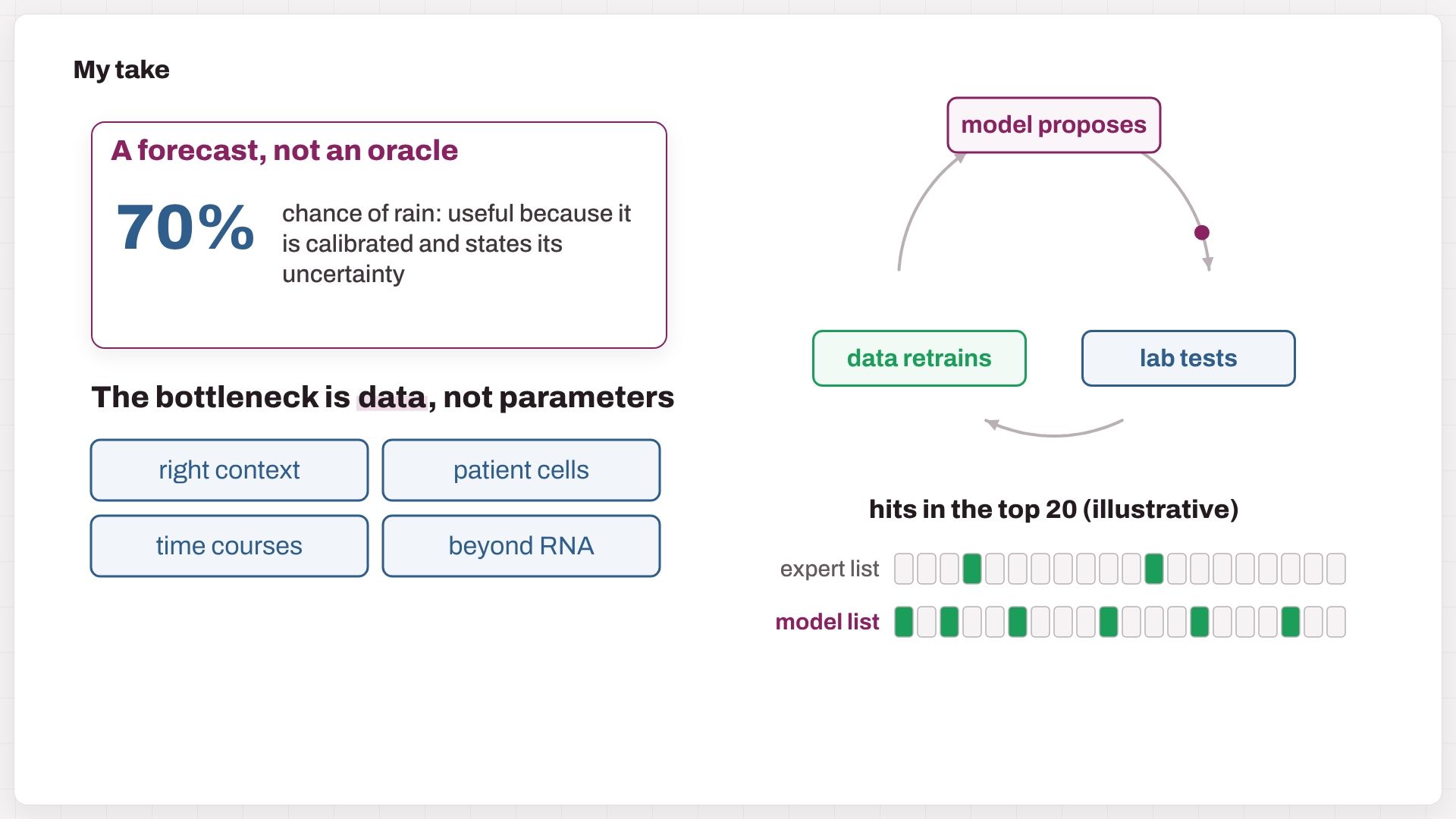
Fig. 8. A forecast rather than an oracle; data as the bottleneck; the lab-in-the-loop; and the one test that matters (the hit counts are illustrative).
- Treat a virtual cell like a weather forecast. It will never be perfect, but it is valuable when it is calibrated and says how uncertain it is. I would rather have a model that says “70%, low confidence for this cell type” than one that is confidently wrong.
- The bottleneck is data, not parameters. Most training data still come from cancer lines and one or two time points. Progress will come from perturbations measured in the right context: primary and patient cells, time courses, and readouts beyond RNA (protein, imaging, function). X-Atlas/Pisces and Tahoe-100M point in that direction.
- The winning setup is a loop. The model proposes, the lab tests, and the results retrain the model. Choosing the next experiment well (active learning) is worth more than predicting every gene perfectly.
- Judge it by decisions, not by correlations. The test that matters is prospective: does the model’s top 20 contain more real hits than your best biologist’s list?
- Expect narrow wins first. I expect the first reliable wins in data-rich, well-defined settings: CRISPR target triage, combination triage, and cell engineering (CAR-T and iPSC protocols), well before a universal human virtual cell.
Try it yourself (Python)
The toy numbers in the video and in Section 8, plus the “average cell” of Fig. 5 (NumPy only):
import numpy as np

rng = np.random.default_rng(685)
G, K = 2000, 60                                    # 2,000 genes, 60 truly change
ctrl = np.clip(rng.normal(4.0, 2.0, G), 0, None)   # control cells: mean log-expression per gene
delta = np.zeros(G)
hit = rng.choice(G, K, replace=False)
delta[hit] = rng.choice([-1, 1], K) * rng.uniform(1.0, 2.2, K)
truth = ctrl + delta                               # what the perturbed cells really look like

preds = {
    "no change":  ctrl.copy(),                                   # copy the control
    "good model": ctrl + delta + rng.normal(0, 0.22, G),         # right changes + noise
    "backwards":  ctrl - delta + rng.normal(0, 0.22, G),         # every change flipped
}

def r(a, b):
    return np.nan if a.std() == 0 or b.std() == 0 else np.corrcoef(a, b)[0, 1]

print(f"{'predictor':12s} {'r(expression)':>14s} {'r(change)':>10s}")
for name, p in preds.items():
    print(f"{name:12s} {r(truth, p):14.2f} {r(delta, p - ctrl):10.2f}")

# The average of a split response lands between the two groups
revive, hold = np.array([0.22, 0.70]), np.array([0.80, 0.38])   # map coordinates of the two groups
mean_cell = 0.6 * revive + 0.4 * hold
print("average cell on the map:", mean_cell.round(3))

# predictor     r(expression)  r(change)
# no change              0.99        nan
# good model             0.99       0.80
# backwards              0.96      -0.80
# average cell on the map: [0.452 0.572]
Further reading
- Reviews and perspectives: Bunne et al., How to build the virtual cell with artificial intelligence, Cell 2024 · Dimitrov et al., Interpretation, extrapolation and perturbation of single cells, Nat Rev Genet 2026 · Ma et al., Virtual cells: progress and challenges, Brief Bioinform 2026 · Xing & Song, A world model of the virtual cell, Cell 2026.
- Foundation models: Geneformer · scGPT · scFoundation · TranscriptFormer · Tahoe-x1.
- Perturbation models: scGen · CPA · chemCPA · GEARS · CellOT · CellFlow · State · X-Cell.
- Data and benchmarks: Genome-scale Perturb-seq (Replogle et al., 2022) · Tahoe-100M · Ahlmann-Eltze et al., 2025 · Miller et al., 2026.
The tumor T-cell map, the 60/40 response split, the “illustrative” hit counts, and the 2,000-gene metric example are simulated for teaching; the script above reproduces the metric numbers. Model scales and licenses are as reported by the authors or repositories at the time of writing and may change. The figures are frames from the video. The video was animated with Remotion and narrated with a synthetic (text-to-speech) voice. Music: “Deliberate Thought” by Kevin MacLeod (incompetech.com), licensed under CC BY 4.0.