In one sentence: DESeq2 puts every sample on a common scale, learns how much each gene normally wobbles between donors, compares each donor with itself, and returns two numbers per V gene: log2FC (how big the change is) and padj (how sure we are that it is more than normal wobble).
\[\text{reads} \approx \text{sample depth} \times \text{donor baseline} \times \text{CAR-T effect}\]padj < 0.05 means “beyond the gene’s normal wobble, after correcting for testing 48 genes”. It does not mean large, important, or consistent in every donor.
These are my working notes from a long series of discussions about one experiment. I kept every question that took more than one round to answer correctly, because those were the places where intuition failed. The video above gives the three-minute version. This page is the full version: the principle, the workflow, the decision rule, how to talk about the results, and the questions and answers.
The experiment. A CAR-T product targets TCR Vβ9 (TRBV9). We ran bulk TCR-seq on CAR-T cells and on untransduced (UTD) control T cells from three donors, with two technical-replicate libraries per sample: 12 libraries, read counts only, no UMIs. We want to answer two questions:
- Is the target, TRBV9, depleted?
- Did any other V gene change (an off-target effect)?
All numbers below come from a simulated data set built to mirror this design (TRBV9 depleted about 97%, one other gene, TRBV12-3, reduced about 30%, everything else unchanged). The script at the end reproduces every number, and the same numbers appear in the video.
1. Why not just compare percentages?
The obvious approach is to compute each V gene’s share of reads in CAR-T and UTD and compare. Four things make that misleading.
- Sequencing depth differs. One library has 0.8 million reads, another 2.5 million. Raw counts are not comparable.
- Proportions are linked. All V genes add up to 100%. When TRBV9 (about 5% of the repertoire) disappears, every other V gene’s share rises by about 6% even though nothing happened to those cells. This is the compositional effect, and a naive comparison reports it as a widespread “increase”.
- Donors differ at baseline. TRBV9 is 3.4%, 3.7% and 9.0% of UTD reads in the three donors. A pooled average mixes donor differences with the treatment effect.
- Three donors and 48 genes. With n = 3 per group, variance estimates are shaky, and with 48 genes some will look different by luck alone.
DESeq2 addresses each of these: size factors handle depth and composition, the donor term handles baselines, dispersion shrinkage stabilises the variance, and the Benjamini–Hochberg correction handles the 48 tests.
2. Before DESeq2: technical replicates and the noise floor
Check the replicates first. The two libraries from the same tube should agree closely (here r = 0.995–0.997 on log CPM), and each library’s nearest neighbour should be its own twin. A library that clusters with another sample signals a swap or a failed prep.
Then sum them. Technical replicates measure the same cells twice. Treating them as independent samples (pseudoreplication) doubles n without adding biological information and makes p-values far too small. Sum the two libraries per sample, so DESeq2 sees 6 samples: 3 donors × 2 conditions.
But first, use them to measure technical noise. For every sample and gene, compute \(\log_2(\text{prep 1}/\text{prep 2})\) on CPM. With 6 samples × 48 genes this gives 288 differences (Fig. 1). Their middle 95% runs from −0.23 to +0.24, so we set the noise floor at N = 0.24 log2, about an 18% change. A change smaller than this cannot be told apart from library-prep and PCR noise.
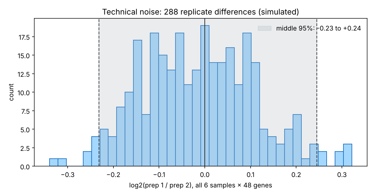
Fig. 1. Technical noise: the log2 ratio between the two libraries of each sample, for all 6 samples × 48 genes (simulated). The shaded middle 95% defines the noise floor.
Two notes on the noise floor:
- It is a reference range for single measurements, not a confidence interval for a mean.
- On the log2 scale it is symmetric, in percent it is not: −N is about a 15% drop (\(2^{-0.24}=0.85\)) and +N an 18% rise (\(2^{0.24}=1.18\)).
Why bother, if DESeq2 already models noise? After summing, DESeq2 never sees the technical replicates. Without UMIs, PCR jackpots can make one library’s V gene jump, and the model may not absorb that fully. The noise floor is an external ruler that DESeq2 does not have. Technical replicates are therefore still worth doing even though they are merged: they provide QC, they define the noise floor, and they protect you from a single bad library.
3. Inside DESeq2: five steps
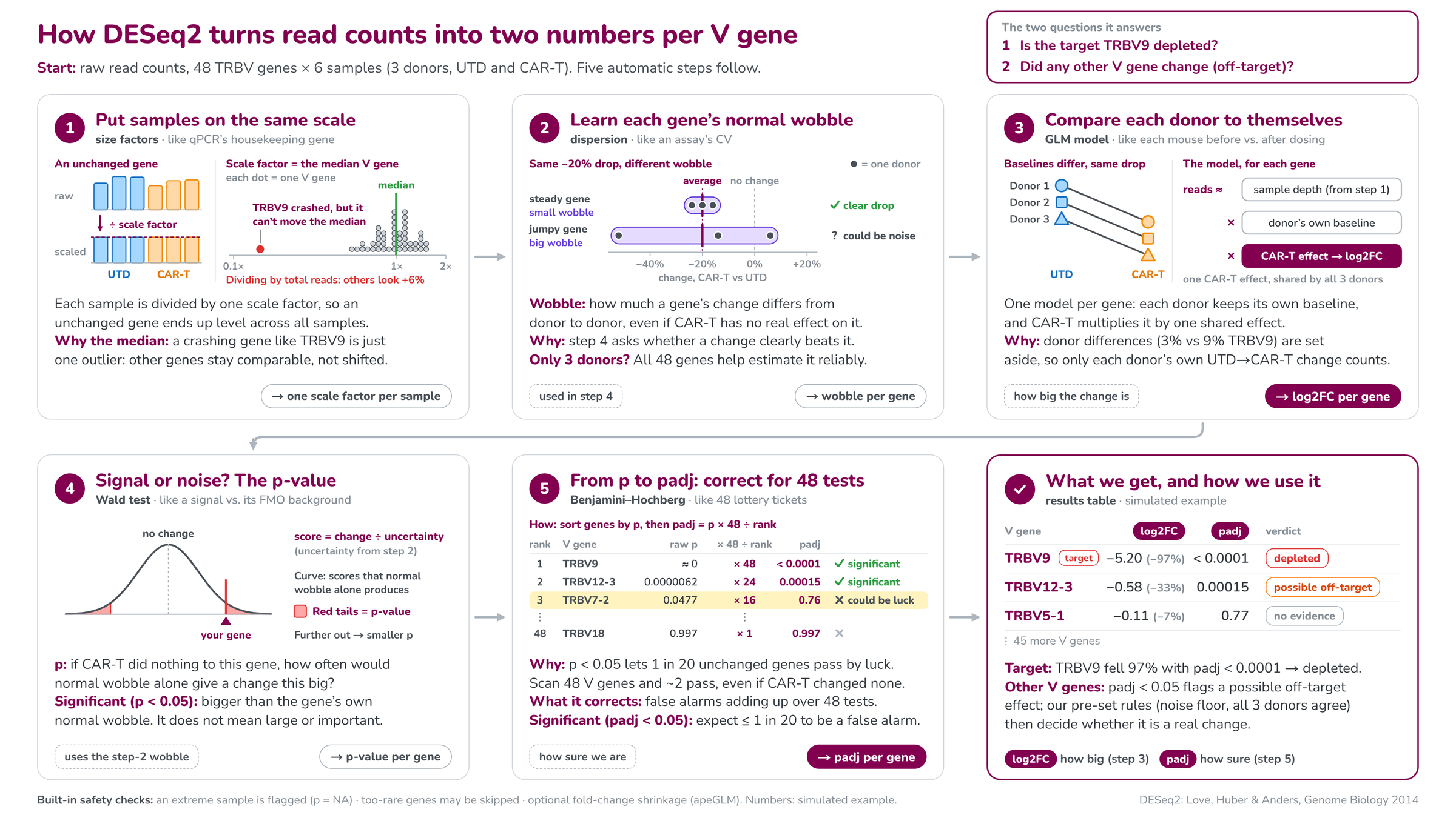
Fig. 2. The five automatic steps from raw counts to log2FC and padj, written for non-statisticians (simulated example). Step 1 makes samples comparable, step 2 provides the yardstick, step 3 estimates the effect, step 4 asks whether it beats the yardstick, step 5 corrects for testing 48 genes.
Step 1. Put samples on the same scale (size factors)
For each gene, DESeq2 computes the geometric mean across all samples as a pseudo-reference. For each sample it divides every gene by that reference and takes the median of these ratios. That median is the sample’s size factor:
\[s_j=\operatorname{median}_i \frac{K_{ij}}{\left(\prod_{v} K_{iv}\right)^{1/m}}\]Each sample’s counts are divided by its size factor. An unchanged gene then comes out level across samples, like normalising qPCR to a housekeeping gene, except the “housekeeping gene” is the typical V gene.
Why the median matters here. TRBV9 crashes in CAR-T samples, but it is one gene out of 48, so it cannot move the median. Normalising by total reads instead would make the other 47 genes look about 6% higher in CAR-T. Median-of-ratios avoids that, under one assumption: most V genes do not change.
In the simulation the size factors are 0.84–1.10. In PyDESeq2 they live in dds.obs["size_factors"].
Step 2. Learn each gene’s normal wobble (dispersion)
DESeq2 models counts with a negative binomial distribution:
\[\operatorname{Var}(K)=\mu+\alpha\mu^2\]The first term is counting (Poisson) noise; the second is biological variation between donors, scaled by the dispersion α. The quantity \(\sqrt{\alpha}\) is the biological coefficient of variation, so a wet-lab analogy is “the assay’s normal CV”. In the simulation the median α is 0.0114, a typical wobble of about 11%.
With only three donors, each gene’s own estimate is rough. DESeq2 therefore runs three sub-steps:
- Gene-wise estimate from that gene alone.
- Trend: fit how dispersion depends on mean expression across all genes.
- Shrinkage: pull each gene’s estimate toward the trend (a maximum a posteriori estimate). Genes with little information move more, genes with strong evidence move less. Genes far above the trend are not shrunk, so a genuinely noisy gene keeps its high dispersion.
The gene-wise, fitted and final values are in dds.var["genewise_dispersions"], dds.var["fitted_dispersions"] and dds.var["dispersions"].
Why this step matters: the wobble is the yardstick used in step 4. The same 20% drop is convincing for a steady gene and noise for a jumpy gene.
Step 3. Compare each donor with itself (the model)
For each gene DESeq2 fits a generalised linear model with the design ~ donor + condition:
Each donor keeps its own baseline, and CAR-T multiplies it by one shared effect. The coefficient \(\beta_{\text{CAR-T}}\) is the log2 fold change. Donor differences (3% vs 9% TRBV9) are set aside, and only each donor’s own UTD → CAR-T change counts.
Two things we verified on the simulated data:
- log2FC is essentially the average of the three per-donor log2FCs. For TRBV9 the model gives −5.201 and the per-donor mean is −5.200; the donors carry 33.1%, 33.3% and 33.6% of the weight. Weights become unequal only when counts are low, because noisier donors get less weight.
- The donor term mainly shrinks the standard error. Without it (
~ condition), the estimate becomes a ratio of pooled means, the SE grows 2–4 times, and TRBV12-3 goes from padj = 0.00015 to padj = 0.999. Pairing is the strongest feature of this design; use it.
PyDESeq2 stores coefficients in dds.varm["LFC"] on the natural log scale; DeseqStats reports log2.
Step 4. Signal or noise? The Wald test and the p-value
The Wald statistic divides the change by its uncertainty, and the p-value comes from the standard normal distribution:
\[z=\frac{\text{log2FC}}{\text{SE}}, \qquad p = 2\,\bigl(1-\Phi(\lvert z\rvert)\bigr)\]For TRBV9, z = −5.20 / 0.135 = −38.5, so p is effectively zero. For TRBV12-3, z = −4.52 and p = 6.2 × 10⁻⁶.
In plain words, p answers: if CAR-T did nothing to this gene, how often would normal wobble alone produce a change this big? Significant (p < 0.05) means the change is bigger than the gene’s own normal wobble. It does not mean the change is large or biologically important.
Step 5. From p to padj: correct for 48 tests
Why. p < 0.05 lets 1 in 20 unchanged genes pass by luck. Scan 48 V genes and about 2 (48 × 0.05 = 2.4) pass even if CAR-T changed none of them.
What is corrected. False alarms adding up over 48 tests. p controls the error per gene; padj controls the error in the final list.
How (Benjamini–Hochberg). Sort genes by p, then padj = p × 48 ÷ rank (plus a step that keeps padj from decreasing down the list):
| Rank | V gene | raw p | × 48 ÷ rank | padj | Call |
|---|---|---|---|---|---|
| 1 | TRBV9 | ≈ 0 | × 48 | < 0.0001 | significant |
| 2 | TRBV12-3 | 0.0000062 | × 24 | 0.00015 | significant |
| 3 | TRBV7-2 | 0.0477 | × 16 | 0.76 | could be luck |
| 48 | TRBV18 | 0.997 | × 1 | 0.997 | not significant |
TRBV7-2 passed p < 0.05 but not padj < 0.05. In the simulation it is truly unchanged: a textbook lucky pass.
Significant (padj < 0.05) means: among all genes called significant, we expect at most 1 in 20 to be a false alarm. Note the two “1 in 20”s: for p it is a rate per unchanged gene, for padj it is a rate per significant gene.
Built-in safety checks
- Extreme samples (Cook’s distance). A single sample that dominates a gene’s fit is flagged. With at least 7 replicates per group DESeq2 would replace the outlier; with 3 per group it cannot, so that gene’s p and padj are set to NA.
- Independent filtering. Genes with very low mean counts can be excluded from the BH correction (padj = NA) to gain power. PyDESeq2 skips filtering when the maximum number of rejections is 10 or fewer, which is typical for 48 V genes.
- Fold-change shrinkage (apeGLM).
lfc_shrinkpulls noisy, low-count log2FCs toward zero for ranking and reporting. It does not change p or padj.
4. The workflow in PyDESeq2
The full, runnable script is deseq2-tcrseq-workflow.py (simulation included; replace simulate() with your own count table). Its core:
# technical replicates: measure the noise floor, then SUM (never treat them as donors)
summed = counts.T.groupby(meta["sample"]).sum().T
md = meta.drop_duplicates("sample").set_index("sample").loc[summed.columns, ["donor", "condition"]]
md["condition"] = pd.Categorical(md.condition, ["UTD", "CART"])

dds = DeseqDataSet(counts=summed.T, metadata=md, design="~donor + condition", inference=inf)
dds.deseq2()
st = DeseqStats(dds, contrast=["condition", "CART", "UTD"], alpha=0.05, inference=inf)
st.summary()
res = st.results_df.copy()
st.lfc_shrink(coeff="condition[T.CART]")          # apeGLM; p-values unchanged
res["lfc_shrunk"] = st.results_df.log2FoldChange

# threshold tests: is the loss > 50% / > 90%?  PyDESeq2's lfc_null is SIGNED
def thr(lfc_null):
    s = DeseqStats(dds, contrast=["condition", "CART", "UTD"], lfc_null=lfc_null, alt_hypothesis="less", inference=inf)
    s.summary(); return s.results_df.padj
res["padj_gt50"], res["padj_gt90"] = thr(-1.0), thr(-np.log2(10))
Its output on the simulated data (Python 3.13, PyDESeq2 0.5.4):
replicate differences: n=288, middle 95% -0.23 to +0.24  ->  noise floor N = 0.24 log2 (18%)
size factors: {'D1_CART': 0.84, 'D1_UTD': 0.93, 'D2_CART': 0.99, 'D2_UTD': 1.1, 'D3_CART': 1.03, 'D3_UTD': 1.03}
median dispersion: 0.0114
          lfc_shrunk  change_%   lfcSE     stat  pvalue    padj                     call
TRBV9        -5.1926  -97.2655  0.1349 -38.5458  0.0000  0.0000             5 eliminated
TRBV12-3     -0.5528  -31.8307  0.1274  -4.5199  0.0000  0.0001    7 candidate reduction
TRBV7-2      -0.2372  -15.1628  0.1266  -1.9805  0.0477  0.7624  2 no evidence of change
TRBV12-5      0.1910   14.1545  0.1223   1.6306  0.1030  0.7666  2 no evidence of change
call
2 no evidence of change    46
5 eliminated                1
7 candidate reduction       1
median log2FC of all V genes (compositional check): 0.008
Practical details that cost us time:
- Where things live in PyDESeq2 0.5.x. Size factors are in
dds.obs["size_factors"](notobsm). Dispersions are indds.var[...]. Normalised counts are indds.layers["normed_counts"]. - Threshold tests differ between R and Python. R’s
lfcThreshold=1, altHypothesis="less"becomeslfc_null=-1, alt_hypothesis="less"in PyDESeq2, becauselfc_nullcarries a sign for one-sided tests. - Do not filter by log2FC after the fact. “padj < 0.05, then keep log2FC < −1” never tested whether the loss exceeds 50%. A gene estimated at −1.1 with a confidence interval from −0.4 to −1.8 is not proven to be halved. Put the threshold into the null hypothesis instead.
- Per-donor log2FCs come from the normalised counts, one CAR-T/UTD ratio per donor. They are needed for the donor-consistency check.
5. Reading the results: the questions that needed several rounds
Does DESeq2’s log2FC average the three donors?
Yes, approximately. With ~ donor + condition and good counts, log2FC equals the mean of the three per-donor log2FCs (−5.201 vs −5.200 for TRBV9). It is a mean of log ratios, so it is not the ratio of pooled percentages.
What exactly is “significant” testing?
Whether the average change clearly exceeds the gene’s uncertainty. That uncertainty bundles two things: how consistently the donors move (dispersion) and counting noise (low counts are noisier). It is not a test of biological importance, and it is not a test that every donor agrees.
padj < 0.05 already accounts for noise. Why also use the noise floor?
In principle padj is enough: it says the change exceeds the noise the model estimated. In this design, discount it for four reasons:
- dispersion has only 2 residual degrees of freedom;
- with 48 genes the dispersion trend is less stable than with 20,000;
- without UMIs, PCR jackpots are lumpy noise the negative binomial may not capture;
- the model never sees the technical replicates.
Large effects are unaffected (TRBV9 is significant even if dispersion is underestimated several-fold). The noise floor matters for changes of 0.3–0.6 log2, which is exactly where off-target calls are made.
padj < 0.05 but |log2FC| below the noise floor?
The change is statistically detectable but smaller than library-prep error. Report it as “below the interpretable threshold”, in supplementary material.
padj ≥ 0.05 but |log2FC| above the noise floor?
The average change looks bigger than measurement error, but the donors disagree too much (or the counts are too low) to attribute it to CAR-T. This is not proven, which is different from “no change”. If all three donors move in the same direction, list it as a trend that needs validation.
If padj includes donor consistency, why check the donors separately?
Because padj < 0.05 does not guarantee that every donor agrees. We tested this by changing one gene’s per-donor shifts in the simulation:
| Per-donor log2FC | padj | Lesson |
|---|---|---|
| −0.85, −0.35, −0.21 | 0.028 | significant, but one donor carries most of the effect |
| −1.04, −0.85, +0.14 | 0.043 | significant although one donor goes the other way |
| −1.6, −0.2, +0.1 | 0.81 | strongly inconsistent: not significant |
I first predicted that the last pattern could be significant and was wrong. DESeq2 does not shrink dispersions that are far above the trend, so a very inconsistent gene keeps its large dispersion and its large SE. In plain words: padj tests whether the average change clearly exceeds donor-to-donor variation, and that can be true while one donor disagrees. A non-significant padj means the average change is not clearly larger than the normal variation, so we cannot attribute it to CAR-T.
How does z become a p-value?
Through the standard normal distribution: \(p=2(1-\Phi(\lvert z\rvert))\). An absolute z of 1.96 gives p = 0.05, and 2.58 gives 0.01. With 48 tests and two significant genes, the BH line sits at an absolute z of about 3.08.
How do I compute the noise floor across three donors?
Pool all log2(prep 1/prep 2) values: 6 samples × 48 genes = 288 differences. Plot the histogram and take the middle 95% (Fig. 1). Per-pair 95th percentiles of the absolute difference ranged from 0.21 to 0.26, so pooling is reasonable. Calling it a “95% CI” is wrong; it is a reference range for single measurements.
A gene drops 33%: is that CAR-T or noise?
33% is log2FC = −0.58. Compare it with the noise floor (0.24): it is more than twice as large. Then check padj (0.00015 for TRBV12-3) and the per-donor values (−0.79, −0.49, −0.45: all three down, all beyond N). That combination supports a real reduction. A 33% drop with padj ≥ 0.05 would be “inconclusive”, and a 15% drop would be inside the noise floor whatever its padj.
Does the same reasoning apply to log2FC = −0.3?
Yes. −0.3 is a 19% drop, just beyond the floor of 0.24. It needs padj < 0.05 and all three donors moving down beyond N before I would call it. Small decreases are also more credible than small increases: the compositional effect pushes non-target genes up, so a decrease appears against that headwind, while an increase of the same size matches the direction and size of the artefact.
Is there a log2FC cut-off that means “eliminated”?
Use −3.32 (a 90% loss) for “eliminated” and −1 (50%) for “strongly reduced”, but test them as hypotheses: lfc_null=-3.32 and lfc_null=-1 with alt_hypothesis="less". Only padj_gt90 < 0.05 supports the word “eliminated”. A log2FC of −1 means halved, not eliminated.
| log2FC | CAR-T / UTD | Reduction |
|---|---|---|
| −0.30 | 0.81 | 19% |
| −0.58 | 0.67 | 33% |
| −1.00 | 0.50 | 50% |
| −2.00 | 0.25 | 75% |
| −3.32 | 0.10 | 90% |
| −4.32 | 0.05 | 95% |
| −6.64 | 0.01 | 99% |
What QC and cut-offs does DESeq2 apply on its own?
Size factors (depth and composition), dispersion shrinkage, Cook’s-distance outlier flagging (p = NA when it cannot replace with 3 per group), independent filtering of very low-count genes (padj = NA; skipped in PyDESeq2 when there are 10 or fewer rejections), and optional apeGLM shrinkage of log2FC. There is no fixed count threshold: independent filtering picks its own cut-off on mean counts to maximise discoveries.
Do low-abundance genes end up with padj ≥ 0.05?
Often, even when the true change is not small. The relative counting noise per sample is about \(\sqrt{1/\mu+\alpha}\), so with α ≈ 0.011 the same 30% drop (log2FC −0.51) behaves very differently:
| Reads per sample | Relative noise (CV) | SE of log2FC | z | p |
|---|---|---|---|---|
| 50,000 (common V gene) | about 10% | 0.12 | 4.2 | < 0.001 |
| 20 (rare V gene) | about 25% | 0.29 | 1.8 | about 0.08 |
| 5 | about 46% | 0.54 | 0.95 | about 0.34 |
apeGLM also shrinks low-count log2FCs toward zero, so a rare gene can fall inside the noise floor as well. Report baseMean alongside the calls, and label rare V genes in classes 2 or 3 as “low abundance, limited power”.
Why doesn’t “padj ≥ 0.05 and |log2FC| ≤ N” prove that nothing changed?
Both conditions look at the centre of the estimate; neither limits how big the true change could be. Example (hand calculation): gene X truly drops 25% (log2FC −0.415), but the donors show −0.80, −0.15 and +0.35. The mean is −0.20 (inside ±0.24), SE = 0.33, z = −0.6, p ≈ 0.55, and the 95% range is −0.85 to +0.45 (a 45% loss to a 37% gain). Gene Y truly unchanged shows −0.05, +0.02 and −0.03: mean −0.02, SE 0.021, 95% range −0.06 to +0.02. Both land in class 2. Only Y has evidence of no change. Noisy data make class 2 more likely, so landing there cannot be evidence of absence.
To claim “no change beyond measurement error”, run an equivalence test, lfc_null=N, alt_hypothesis="lessAbs": padj < 0.05 means the whole uncertainty range lies within ±N. Otherwise, write “no change detected”.
6. A reusable decision rule for every V gene
Five criteria, each answering a different question:
| Question | Criterion |
|---|---|
| Beyond donor-to-donor variation? | padj < 0.05 |
| Beyond measurement error? | |log2FC| > N (noise floor) |
| Supported by every donor? | all three donors in the same direction; each donor’s change beyond N (otherwise flag “magnitude inconsistent”) |
| How large? | threshold tests: > 90% = eliminated, > 50% = strongly reduced, otherwise candidate |
| An increase? | consider the compositional effect first |
Applied in order, every gene lands in exactly one of eight outcomes (Fig. 3).
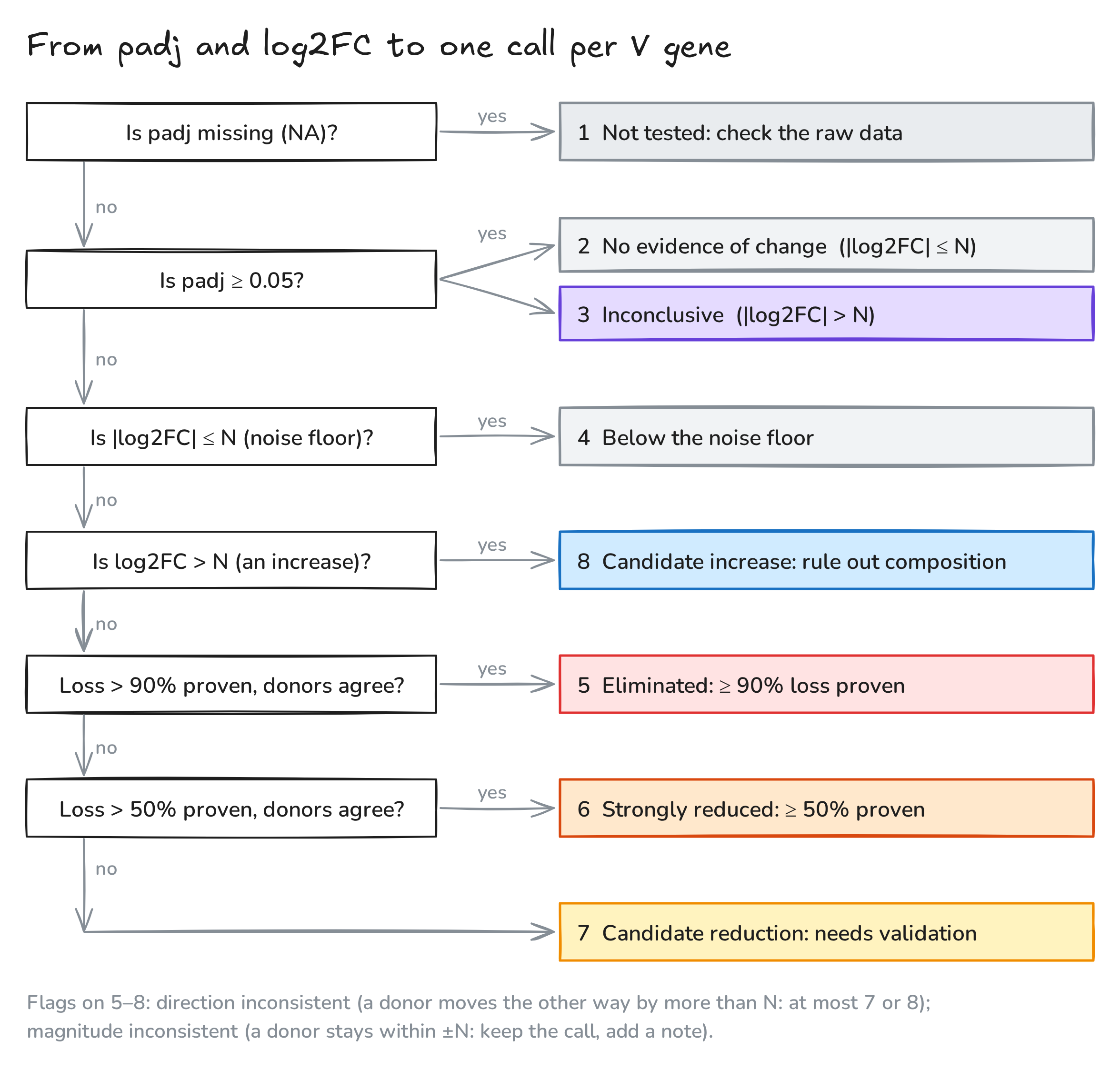
Fig. 3. From padj and log2FC to one call per V gene. Each question is asked in order; the first “yes” decides the class.
| Outcome | Condition | Meaning and how to report |
|---|---|---|
| 1 Not tested | padj = NA | DESeq2 gave no result (an extreme sample was flagged, or too few reads). Report “not evaluable” and inspect the donors’ raw data |
| 2 No evidence of change | padj ≥ 0.05, |log2FC| ≤ N | “No change detected”, which is not proof of no change |
| 3 Inconclusive | padj ≥ 0.05, |log2FC| > N | Not proven, not “no change”. If all three donors agree in sign, list as a trend to validate |
| 4 Below the noise floor | padj < 0.05, |log2FC| ≤ N | Stable but smaller than library-prep error. Supplementary: “below the interpretable threshold” |
| 5 Eliminated | padj < 0.05, log2FC < −N, > 90% test significant, no opposite donor | Loss ≥ 90% proven. Main finding |
| 6 Strongly reduced | as 5, but only the > 50% test is significant | Loss ≥ 50% proven, ≥ 90% not. Main text |
| 7 Candidate reduction | padj < 0.05, log2FC < −N, not 5 or 6 | A real decrease whose size is not proven to exceed half. Results table, “needs validation” |
| 8 Candidate increase | padj < 0.05, log2FC > N | Rule out the compositional effect first. Results table with a caution |
A gene reaches class 7 in three ways: the estimate is below 50%; the estimate is above 50% but the threshold test is not significant (wide uncertainty); or the donors disagree in direction.
Two flags on classes 5–8.
- Direction inconsistent: a donor moves the other way by more than N. Such a gene can be at most 7 or 8.
- Magnitude inconsistent: all donors agree, but at least one donor’s change stays within ±N, so two donors carry the effect. Keep the class and add the note.
To keep the flags from overlapping, classify each donor as down (< −N), flat (within ±N) or up (> N). The sign of a flat donor is noise, so it should raise “magnitude inconsistent”, not “direction inconsistent”. A plain sign check (all three log2FCs negative) gets this wrong.
Class 8, the increases. TCR-seq measures proportions, so a rising share can mean real expansion or simply that other cells left. Check the median log2FC of all V genes (0.008 here): a clearly positive median means everything was pushed up and small increases should be discounted. An increase similar to that shift is “possibly compositional”. An increase well beyond it, with all three donors up and each beyond N, is “relative enrichment”, which needs flow cytometry with absolute counts to confirm. An increase is never off-target killing: CAR-T killing can only reduce a V gene.
Reading the classes for the two questions.
- Q1, the target TRBV9. 5 = depleted. 6 = partially depleted (≥ 50% proven, ≥ 90% not). 7 = reduced, extent uncertain. 2, 3 or 4 = depletion not demonstrated: check CAR-T function and the experiment. 1 = check the data.
- Q2, other V genes. 5 or 6 = strong off-target signal; express it as a percentage of TRBV9’s effect. 7 = possible off-target, validate. 8 = not off-target killing, most likely compositional. 2 or 4 = no evidence of off-target. 3 = cannot be excluded, list for validation. 1 = not evaluable.
In the simulation: TRBV9 is class 5, TRBV12-3 is class 7 (−32%, padj 0.00015, all three donors down beyond N), and the other 46 genes are class 2.
7. Explaining it to wet-lab colleagues
Stakeholders want two answers: “was the target removed?” and “was anything else hit?”. What worked for us:
- Lead with the question, then the number. “TRBV9 fell 97% in every donor (padj < 0.0001): depleted.” “One other V gene, TRBV12-3, fell about 32%; it passes our pre-set rules for a candidate and we will validate it by flow.”
- Translate log2FC into percent, using the table in section 5.
- Explain padj in one line: “how sure we are that the change is bigger than normal donor-to-donor variation, after allowing for testing 48 genes”.
- Use the analogies in Fig. 2: size factors as qPCR’s housekeeping gene; dispersion as an assay’s CV; the paired model as each mouse measured before and after dosing; the Wald test as a signal against its FMO background; multiple testing as buying 48 lottery tickets.
- Report absolute frequencies too. log2FC is relative; “TRBV9 went from 5.4% to 0.16% of reads” is the most direct evidence of depletion.
- Use TRBV9 as a yardstick. An off-target gene reaching 70–100% of TRBV9’s effect suggests cross-recognition; 10–20% is more likely indirect or compositional.
- Pre-register the rules. Write the noise floor, thresholds and donor rules into the methods before looking at results.
8. Is DESeq2 appropriate for TCR-seq?
Yes, with conditions. What it tests here is differential abundance of V-gene usage, not expression. The data have the same shape as RNA-seq (integer counts, samples × features), the negative binomial handles count noise, median-of-ratios handles depth and a single strongly changing gene, and the paired design is used directly. On the simulated data it recovered TRBV9 and TRBV12-3 with no false calls among the other 46 genes.
The conditions and limits:
- Most V genes must be unchanged. If many change, normalisation is biased. Check the median log2FC.
- Reads are not cells. In RNA-based TCR-seq, TCR transcripts per cell change with activation; gDNA-based TCR-seq is closer to cell numbers. Either way the conclusion is about proportions; confirm cell loss by flow.
- No UMIs. PCR bias and jackpots exist. V-primer efficiency differences largely cancel in fold changes when both groups use the same protocol, but the noise floor is needed.
- 48 features. Dispersion sharing works less well than with 20,000 genes, so be careful with small effects.
- Three donors. Power is limited, so “not significant” means “not detected”.
Is it trusted, and are there precedents? DESeq2 is one of the most cited methods in genomics (Love et al. 2014), and benchmarking work has recommended DESeq2 or edgeR when replicates are few. For immune repertoires there is no gold standard. From a literature search:
- Closest precedent: Malik et al. (PLOS ONE 2022) used edgeR, which shares the negative-binomial framework, for differential TRBV usage on bulk multiplex-PCR TCR-seq processed with MiXCR. That is almost exactly this setting.
- Clonotype-level uses: edgeR (Pollastro et al., Front Immunol 2021, UMI-corrected clone counts) and a modified DESeq (Cha et al., Sci Transl Med 2014).
- A caution: a 2025 bioRxiv preprint (Buytenhuijs et al.) reports that DESeq2 and edgeR can be anti-conservative on sparse clonotype-level data. V-gene counts are dense, so the concern is much smaller here. It is still the reason for the extra noise-floor and donor rules.
- What most repertoire papers do: paired t-tests, Wilcoxon or MANOVA. There is also a dedicated Bayesian tool, IgGeneUsage.
- No direct precedent found: I did not find a published study that used DESeq2 specifically for V-gene usage.
A defensible methods sentence:
V-gene usage was compared with DESeq2 (Love et al., 2014; PyDESeq2, Muzellec et al., 2023) using a paired design (~donor + condition) after summing technical replicates. Because count-based methods can be anti-conservative on repertoire data, significant genes also had to exceed a technical-replicate noise floor and agree across all three donors; results were cross-checked with edgeR.
9. Lessons I would pass on
- Design is half the analysis. Paired donors plus technical replicates gave both the donor term and the noise floor.
- Sum technical replicates; never count them as donors.
- Always put donor in the design. It turned TRBV12-3 from padj 0.999 into 0.00015.
- Measure your own noise floor from the replicates before looking at fold changes.
- Test thresholds; do not filter after the fact.
- padj is necessary, not sufficient. Read it together with the noise floor, the per-donor values and the threshold tests.
- “Not significant” is not “no change”. Use an equivalence test if you need to claim absence.
- Treat small increases with suspicion: they match the compositional artefact.
- Low-abundance genes have little power. Show baseMean and say so.
- Write the rules down before the results arrive, and validate candidates orthogonally (flow cytometry with Vβ antibodies, more donors) rather than with more statistics.
- Verify claims with a simulation. Several intuitive answers in this series (including mine) were wrong until we changed the data and re-ran the model.
Notes. All data are simulated for teaching (seed 1): 48 TRBV genes, 3 donors, 2 conditions, 2 technical-replicate libraries per sample, multinomial sampling of 0.8–2.5 million reads per library, donor-to-donor variation (SD 0.35 on the log scale), culture drift (0.10) and library-prep noise (0.06); TRBV9 retained at 3% and TRBV12-3 at 70% in CAR-T. The per-donor inconsistency examples were made by editing one gene’s simulated shifts and re-running the model; the gene X / gene Y and low-count tables are hand calculations. The runnable workflow is deseq2-tcrseq-workflow.py. Fig. 3 and the graphical abstract were drawn with Excalidraw; the editable sources: abstract, Fig. 3. The video was animated with Remotion and narrated with a synthetic (text-to-speech) voice. Music: “Deliberate Thought” by Kevin MacLeod (incompetech.com), licensed under CC BY 4.0. Created by Miao Li.*
References. Love MI, Huber W, Anders S (2014). Moderated estimation of fold change and dispersion for RNA-seq data with DESeq2. Genome Biology 15:550. Muzellec B, Teleńczuk M, Cabeli V, Andreux M (2023). PyDESeq2: a python package for bulk RNA-seq differential expression analysis. Bioinformatics. Benjamini Y, Hochberg Y (1995). Controlling the false discovery rate. J. R. Stat. Soc. B 57:289–300. Zhu A, Ibrahim JG, Love MI (2019). Heavy-tailed prior distributions for sequence count data (apeglm). Bioinformatics 35:2084–2092. Malik A et al. (2022). Distorted TCR repertoires define multisystem inflammatory syndrome in children. PLOS ONE 17:e0274289. Pollastro S et al. (2021). Characterization and monitoring of antigen-responsive T cell clones using T cell receptor gene expression analysis. Front. Immunol. 11:609624. Cha E et al. (2014). Improved survival with T cell clonotype stability after anti–CTLA-4 treatment in cancer patients. Sci. Transl. Med. 6(238). Buytenhuijs F et al. (2025). Differential T cell receptor clonotype abundance analysis with similarity-based counts weighting. bioRxiv. IgGeneUsage, Bioconductor.