A guided reading of Bender et al., “Artificial intelligence in drug discovery — what it is, where we stand and the path forward”, Nature Reviews Drug Discovery (2026), doi:10.1038/s41573-026-01496-2.
In one sentence: AI has given drug discovery impressive tools but still little proof of clinical impact; to change that, aim models at the decisions that matter in the clinic, feed them data that predict human outcomes, and judge them by better decisions, not better benchmarks.
The video above and this walkthrough follow the paper, a Perspective by sixteen researchers who take stock of a decade of AI in drug research, in eight steps. Two numbers are our own: a re-run of the classic cost model the authors build on, and a small demo of their point about metrics. The code for both is at the end.
1. The scorecard
The technology has clearly advanced: protein structures can be predicted, proteins can be designed, and new measurement technologies produce more data than ever. The clinical record is thinner. In the pipelines of AI-first drug companies, most projects are still preclinical, several dozen have reached phase I or II, and only a handful phase III. Reports of phase I success rates of up to 90% exist, but most of those molecules act on well-understood biology, where safety surprises are rarer. The authors’ verdict is careful: so far this is an absence of evidence, not evidence that AI cannot help.
2. Where the value hides
Suppose AI made one stage of drug development 20% faster, 20% cheaper or 20% less likely to fail. Which change saves the most per approved drug? We re-ran the classic R&D cost model (Paul et al., 2010) that the authors build on. It reproduces the familiar $1,778M capitalized cost per approved drug, and the answer is unambiguous: cutting phase II failures by a fifth saves about $396M, far more than any other change. Phase II is where a drug is first tested for efficacy in patients, and most candidates fail there.
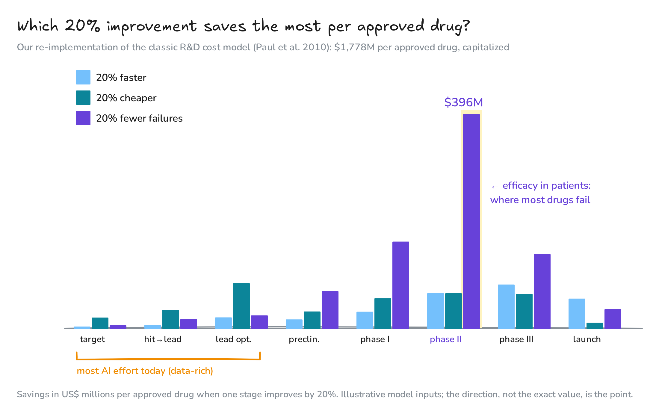
Fig. 1. Savings per approved drug from 20% improvements at each stage
Yet most AI effort goes into early hit discovery, because that is where labelled data exist. The authors compare this to looking for your keys under the streetlight rather than where you dropped them. The lever that already works is at the clinical end: projects that use biomarkers to select the right patients cost roughly half as much per approved drug, and drug targets with human genetic support are about 2.6 times more likely to succeed.
3. A ligand is not a drug
Press releases often blur two different things. A ligand binds its target in a test tube. A drug must also reach the right tissue, stay stable long enough, avoid off-target harm and help patients at a usable dose. Databases hold more than a million bioactive ligands but only about a thousand approved drugs. Designing better binders is progress in ligand discovery, which is only one early step of drug discovery.
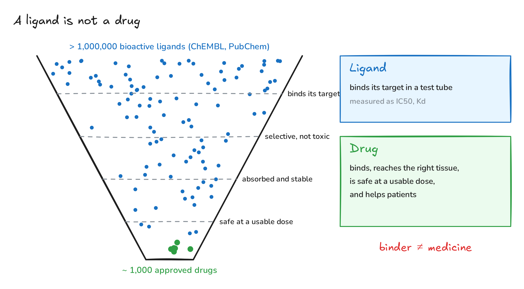
Fig. 2. Many ligands, few drugs
4. Biology is conditional
The same drug does different things in different contexts. Imatinib works remarkably well in leukaemia driven by the Philadelphia chromosome and not in other forms of the same disease. Liver enzymes, smoking, diet and the gut microbiome all change how a patient responds. Even a simple label such as “this compound is active” depends on the assay and its settings. On top of that, cheap proxy assays often correlate only weakly with what happens in patients: the authors show liver organoid toxicity against clinical liver injury, and a thermal-shift binding assay against enzyme inhibition. A model trained on such data inherits the weak link. Their recommendation: check how well your data predict the outcome that matters, before and after you build a model.
5. Chemistry is a universe of small islands
Chemical space holds around \(10^{60}\) drug-like molecules; any dataset is a small, biased island in it. Four widely used public ADME datasets share just 0.1% of their compounds, so models for solubility, permeability, brain penetration and clearance are trained on different islands, which makes multi-property optimization shaky. Random train–test splits keep test molecules close to the training set, so reported scores overestimate performance on the next project, which usually sits in a different “galaxy”. Biased data can even fool explainable AI: one model decided that sugar rings make molecules taste bitter, because many bitter natural products happen to carry sugars.
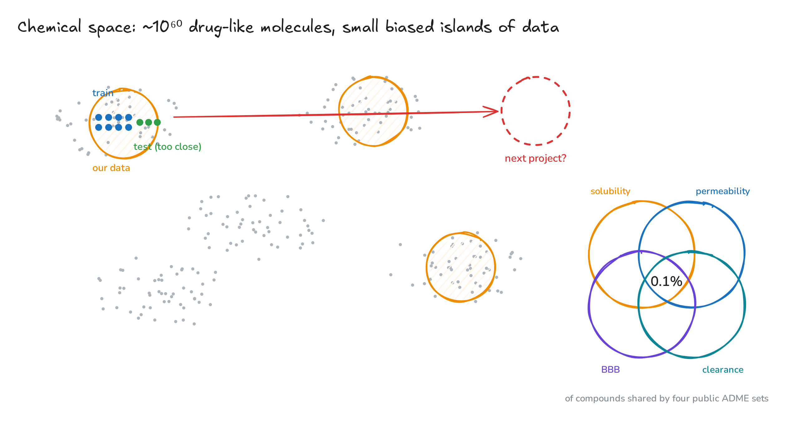
Fig. 3. Datasets are small islands in chemical space
6. Same score, different jobs
How a model is judged should depend on how it will be used. In a selection setting (picking hits from a huge library) what matters is how many actives land at the top of the list. In a deselection setting (filtering out toxic or unstable compounds) what matters is how few bad compounds slip through. In a quantification setting (predicting a human dose) what matters is the error in real units. A single summary number such as the AUC hides all of this. Our two illustrative models have exactly the same AUC, 0.74, yet model A finds 45% of the actives in the top 10% (model B: 26%), while model B lets only 1.0% of toxic compounds through a filter that discards the riskiest 80% (model A: 7.5%).
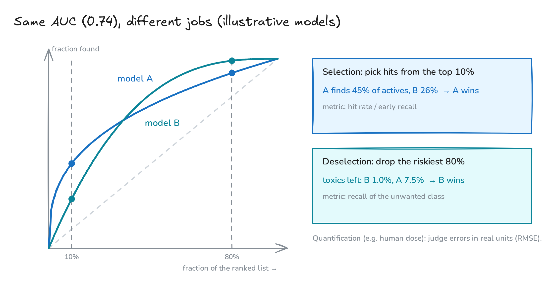
Fig. 4. Two models with the same AUC and opposite strengths
The same logic applies to benchmarks in general: when a benchmark becomes the target, it stops measuring progress (Goodhart’s law), and chasing state-of-the-art numbers on generic datasets can create an illusion of progress.
7. Models live in processes
A model never works alone. Before it comes the project context: the target organ, the disease subtype, the dose that will be reached in humans. After it come the follow-up experiments and, eventually, a decision. Validating the model on a test set checks only the middle box. What matters is whether the whole process makes better decisions. The authors summarize a model’s worth in one line:
\[\text{model value}=\Delta\,\text{clinical success rate}\times\text{project applicability domain}\]A model that improves clinical success a little, across many projects (for example a pharmacokinetics or safety model), can be worth more than a spectacular model for one target.
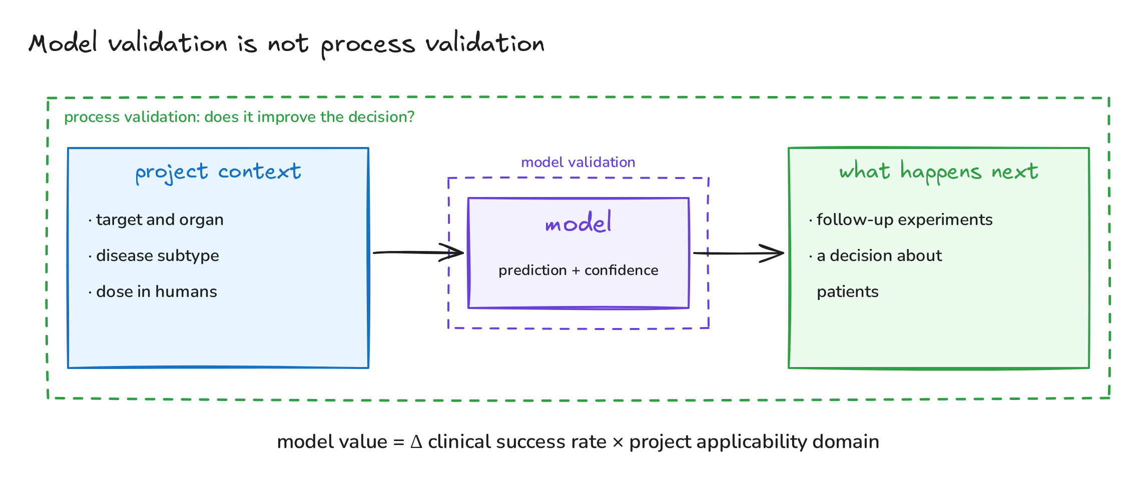
Fig. 5. Model validation is only the middle of the process
8. The path forward
- Generate the right data first. Explore which cheap assays actually predict human efficacy and safety, then scale those up and build production models with a known applicability domain.
- Use human-relevant systems with rich readouts: primary cells from many donors, stem-cell-derived neurons, organoids, co-cultures, measured with Cell Painting or single-cell sequencing.
- Learn from the clinic. Break the wall between preclinical and clinical data so that models learn from real outcomes, including failures.
- Build purpose-made data together, for example consortia with harmonized assays, or public efforts such as OpenADMET (ARPA-H funded, $30M).
- Mind the incentives. Rising R&D costs, bold promises and publication pressure all reward impressive numbers over real impact.
The paper ends with a simple test for success: not better benchmarks, but more approved drugs and genuinely new medicines.
What to take away
- If you build models: start from the decision the model will support, choose the metric for that decision, and test on chemistry and biology the model has not seen.
- If you run drug projects: ask how well each dataset predicts the clinical outcome, and invest where failures are most expensive: efficacy in patients.
- If you are new to the field: AI is a powerful set of tools, not a shortcut; the hard part of drug discovery is still knowing which molecule helps which patient.
Try it yourself (Python)
"""Two small calculations behind the video "AI in drug discovery: where do we really stand?"
1) The classic R&D cost model (Paul et al., Nat Rev Drug Discov 2010), as used by Bender et al. (2026):
   which 20% improvement saves the most per approved drug?
2) Two screening models with the same AUC but opposite usefulness (illustrative)."""
import numpy as np

stages = ["target-to-hit", "hit-to-lead", "lead opt.", "preclinical", "phase I", "phase II", "phase III", "launch"]
p = np.array([0.80, 0.75, 0.85, 0.69, 0.54, 0.34, 0.70, 0.91])   # probability of success per stage
cost = np.array([1, 2.5, 10, 5, 15, 40, 150, 40.0])               # US$ million per project in the stage
years = np.array([1.0, 1.5, 2.0, 1.0, 1.5, 2.5, 2.5, 1.5])        # duration of each stage
r = 0.11                                                           # cost of capital

def cost_per_launch(p, cost, years, capitalized=True):
    projects = 1 / np.array([p[k:].prod() for k in range(len(p))])     # projects needed per launch
    if not capitalized:
        return (projects * cost).sum()
    t_left = np.array([years[k] / 2 + years[k + 1:].sum() for k in range(len(p))])
    return (projects * cost * (1 + r) ** t_left).sum()               # money spent earlier costs more

base = cost_per_launch(p, cost, years)
print(f"per approved drug: ${cost_per_launch(p, cost, years, False):.0f}M out of pocket, ${base:.0f}M capitalized")
print(f"{'stage':14s} {'20% faster':>11s} {'20% cheaper':>12s} {'20% fewer failures':>19s}")
for k, s in enumerate(stages):
    y, c, q = years.copy(), cost.copy(), p.copy()
    y[k] *= 0.8; c[k] *= 0.8; q[k] = 1 - 0.8 * (1 - p[k])
    print(f"{s:14s} {base - cost_per_launch(p, cost, y):11.0f} {base - cost_per_launch(p, c, years):12.0f} "
          f"{base - cost_per_launch(q, cost, years):19.0f}")

# 2) Same AUC, different jobs: recall curves over a ranked list (x = fraction of the list examined)
g = 0.35
d = 1 / (1 - 1 / (1 + g)) - 1              # chosen so that both curves have the same area
recall_A = lambda x: x ** g                # strong early enrichment
recall_B = lambda x: 1 - (1 - x) ** d      # leaves almost nothing at the bottom of the list
print(f"\nAUC: A = {1 / (1 + g):.3f}, B = {1 - 1 / (1 + d):.3f}")
print(f"pick hits, top 10%:      A finds {recall_A(0.1):.1%} of actives, B finds {recall_B(0.1):.1%}")
print(f"weed out toxics, drop 80%: toxic compounds left: A {1 - recall_A(0.8):.1%}, B {1 - recall_B(0.8):.1%}")
per approved drug: $873M out of pocket, $1778M capitalized
stage           20% faster  20% cheaper  20% fewer failures
target-to-hit            1           19                   4
hit-to-lead              5           33                  16
lead opt.               19           83                  23
preclinical             15           30                  68
phase I                 30           55                 160
phase II                64           64                 396
phase III               80           63                 137
launch                  54           10                  34

AUC: A = 0.741, B = 0.741
pick hits, top 10%:      A finds 44.7% of actives, B finds 26.0%
weed out toxics, drop 80%: toxic compounds left: A 7.5%, B 1.0%
This is an independent summary written for teaching; please read the original paper for the full argument and references. The cost model is our re-implementation of Paul et al. (2010) with its published inputs, not the authors’ updated calculation, so exact values differ from the paper’s Fig. 1; the direction of the result is the same. The two models in Fig. 4 are illustrative, inspired by the paper’s Fig. 5. All figures were drawn by us with Excalidraw; the editable sources open directly on excalidraw.com: Fig. 1, Fig. 2, Fig. 3, Fig. 4, Fig. 5. The video was animated with Remotion and narrated with a synthetic (text-to-speech) voice. Music: “Deliberate Thought” by Kevin MacLeod (incompetech.com), licensed under CC BY 4.0.