In one sentence: GPT learns language by predicting the next token across the internet, learns to follow instructions from human examples, then practices against a reward model built from human rankings, on a KL leash that keeps it close to where it started.
\[\max_{\pi_\theta}\;\mathbb{E}_{x\sim D,\;y\sim\pi_\theta(\cdot\mid x)}\big[r_\phi(x,y)\big]\;-\;\beta\,\mathrm{KL}\big(\pi_\theta(\cdot\mid x)\,\Vert\,\pi_{\text{ref}}(\cdot\mid x)\big)\]The judge is not the truth, and the leash is not a guarantee.
The video above follows one prompt, “Explain vaccines to a six-year-old.”, through all four stages of training. The sizes and results for GPT-3 and InstructGPT come from the two papers (Brown et al. 2020; Ouyang et al. 2022). The tokens are real GPT-3 tokens. The next-token probabilities in section 3 are illustrative. The reward model and the PPO run are a small but real toy, and the script in section 8 reproduces every one of their numbers.
1. Same Transformer, different training
Type our prompt into a raw, pretrained language model and it may just keep going: “Explain antibodies to a six-year-old. Explain fevers to a six-year-old.” On the internet, lines like that come in lists (worksheets, FAQs, homework), so continuing the list is a perfectly good guess for the next tokens. OpenAI showed exactly this behavior for GPT-3 with the prompt “Explain the moon landing to a 6 year old”. An assistant like ChatGPT answers instead: “A vaccine is a practice drill for your body’s defenders.”
Both are Transformers trained on internet text. What changed is the training, in four stages:
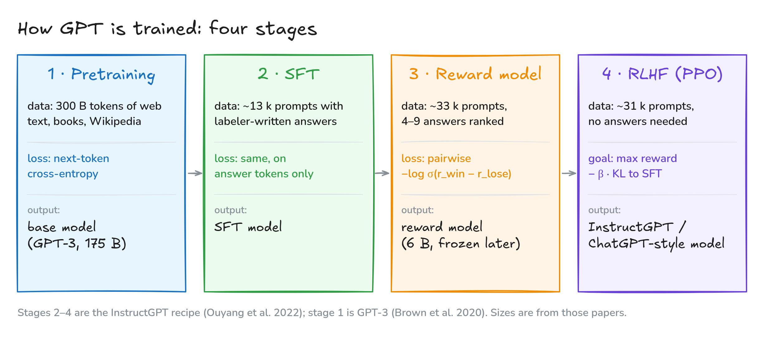
Fig. 1. The four stages: read the internet, copy good examples, train a judge, practice against the judge on a leash.
2. What GPT is
GPT stands for Generative Pre-trained Transformer. It is a decoder-only Transformer (see my Transformer explainer), and it reads text as tokens: pieces of words from a vocabulary of 50,257. The real GPT-3 tokenizer splits Vaccines into three tokens, V · acc · ines (IDs 53, 4134, 1127). GPT has one job: given the tokens so far, output a probability for every possible next token. To write, it picks one, appends it and repeats. This is autoregressive generation. Inside, masked self-attention lets each token look back, never ahead, so training and generation see the same thing.
By the chain rule of probability, a whole text is a product of next-token probabilities:
\[P(w_1,\dots,w_T)=\prod_{t=1}^{T}P_\theta(w_t\mid w_{<t})\]3. Stage 1, pretraining: a guessing game at internet scale
Show the model “Vaccines train your immune” and ask for the next token. Suppose it gives system, the true next word, 62%. The loss for that position is minus the log of that probability:
\[-\log 0.62 = 0.48 \qquad\text{whereas}\qquad -\log 0.05 = 3.0\]A confident right guess costs little, and a confident wrong one costs a lot. Gradient descent nudges every weight so that the true token becomes a little more likely. Averaged over every position in the data, this is the cross-entropy (negative log-likelihood) loss:
\[\mathcal{L}_{\text{LM}}(\theta)=-\frac{1}{T}\sum_{t=1}^{T}\log P_\theta(w_t\mid w_{<t})\]No human labels are needed, because the text is its own answer key. That is what self-supervised means, and it is why pretraining can use the whole internet.
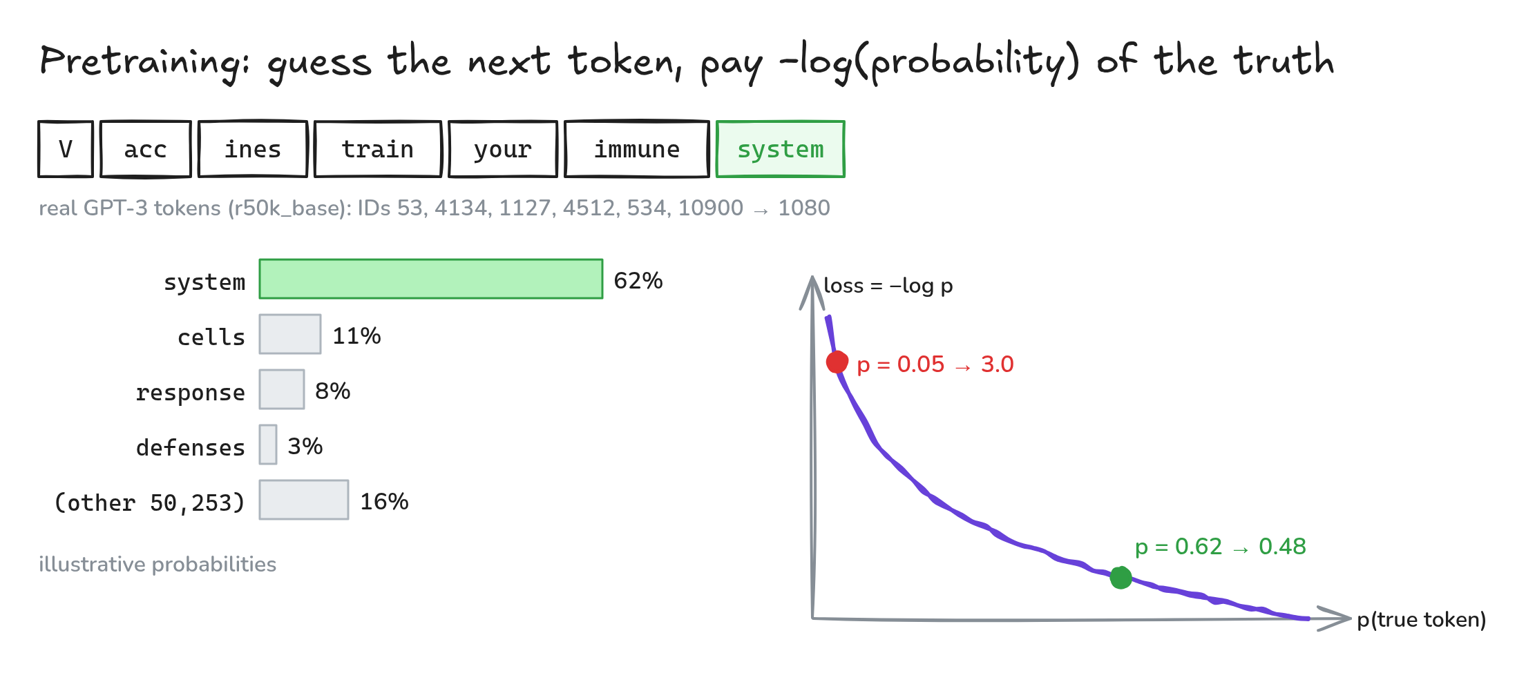
Fig. 2. Left: the model’s guesses (illustrative). Right: the loss −log p. Probability 0.62 on the true token costs 0.48; probability 0.05 costs 3.0.
| GPT-3 (Brown et al. 2020) | |
|---|---|
| Parameters | 175 billion (96 layers, width 12,288, 96 attention heads, context 2,048 tokens) |
| Training tokens | 300 billion |
| Data mix (sampling weight) | Common Crawl, filtered 60% · WebText2 22% · Books1 8% · Books2 8% · Wikipedia 3% |
| Compute | \(\approx 6\,N\,D = 6 \times 175\text{B} \times 300\text{B} \approx 3.1\times10^{23}\) FLOPs (3,640 petaflop/s-days) |
The result is a base model that knows a great deal about grammar, facts, code and styles. But it has only one goal: continue the document.
4. Stage 2, supervised fine-tuning (SFT): copy good examples
A document-continuer imitates the internet, errors, rambling and toxicity included. We want an assistant that is helpful, honest and harmless. So OpenAI hired about 40 labelers to write ideal answers for about 13,000 prompts, for example:
Prompt: Explain vaccines to a six-year-old.
Ideal answer: A vaccine is a practice drill for your body’s defenders. It shows them a harmless “wanted poster” of a germ, so they learn to catch it fast.
SFT uses the same next-token loss, counted only on the answer tokens. The prompt tokens are context, not targets:
\[\mathcal{L}_{\text{SFT}}(\theta)=-\sum_{t\,\in\,\text{answer}}\log \pi_\theta(y_t\mid x,\,y_{<t})\]The SFT model now follows instructions. But great answers are slow and costly to write, and imitation can only be as good as the demonstrations. People are much better at judging answers than at writing them, and that observation drives the next two stages.
5. Stage 3, the reward model: turn rankings into a number
For each prompt, the SFT model writes several answers (4 to 9 in InstructGPT). In our toy example there are four:
| Answer | Note | |
|---|---|---|
| A | A practice drill: your body sees a harmless “wanted poster” of a germ. | clear, kind, correct |
| B | Vaccines deliver antigens that prime adaptive immunity via memory B and T cells. | correct, but jargon |
| C | Explain antibodies to a six-year-old. Explain fevers to a six-year-old. | keeps the list going |
| D | Vaccines are dangerous. Skip them. | false and harmful |
The labeler does not score them. They rank them: A ≻ B ≻ C ≻ D. This resolves a common puzzle: the ground truth is a ranking, the model outputs a number, so how can there be a loss? A ranking of \(K\) answers is really \(\binom{K}{2}\) pairwise comparisons (6 for four answers, 36 for nine), and each pair is a small binary question: should the winner’s number be larger? InstructGPT collected rankings for about 33,000 prompts.
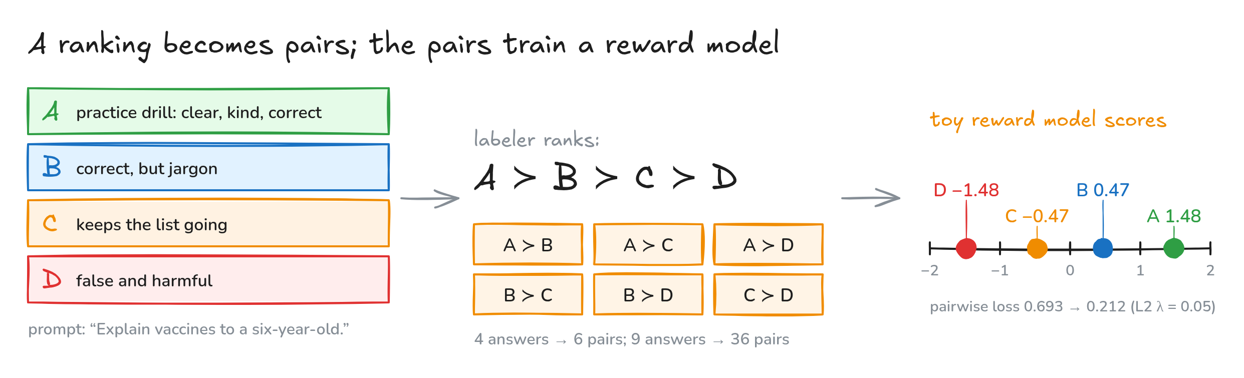
Fig. 3. A ranking unfolds into pairs. Fitting the pairs gives each answer a score. Only differences between scores matter.
Architecture. The reward model is the SFT Transformer with its vocabulary output replaced by a scalar head that reads the hidden state of the last token:
\[r_\phi(x,y)=\mathbf{w}^{\top}\mathbf{h}_{\text{last}}+b\;\in\;\mathbb{R}\]InstructGPT used a 6-billion-parameter reward model.
Loss. The Bradley–Terry model turns two rewards into a probability, the sigmoid of their difference, and the loss is minus its log:
\[P(y_w\succ y_l\mid x)=\sigma\big(r_\phi(x,y_w)-r_\phi(x,y_l)\big),\qquad \mathcal{L}_{\text{RM}}(\phi)=-\log\sigma\big(r_\phi(x,y_w)-r_\phi(x,y_l)\big)\]Write \(\Delta = r_w - r_l\). The gradient is
\[\frac{\partial\mathcal{L}}{\partial\Delta}=\sigma(\Delta)-1 \;<\; 0\]It always raises the winner and lowers the loser, strongly when the order is wrong and hardly at all once the order is clear. In numbers:
- Before training, all rewards are equal: \(\Delta=0\), a coin flip, loss \(\ln 2 = 0.693\).
- After training, the toy judge scores A = 1.48, B = 0.47, C = −0.47, D = −1.48. For the pair A over B, \(\Delta = 1.01\), \(\sigma(1.01)=0.73\), loss 0.31 and gradient −0.27.
- If the order were flipped, the same gap would cost 1.32.
Adding 5 to every score changes nothing, because only differences enter \(\sigma\). (InstructGPT shifts the reward model so that the labelers’ demonstrations average 0.) Over all \(\binom{K}{2}\) pairs of a prompt the loss is averaged with weight \(1/\binom{K}{2}\), and all pairs from one prompt go into a single batch element so that the model does not overfit to that prompt.
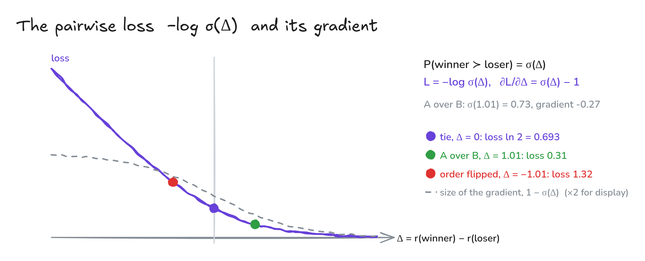
Fig. 4. Tie: 0.693. A over B by 1.01: 0.31. Flipped: 1.32. The dashed curve shows the size of the gradient, which fades as Δ grows.
6. Stage 4, RLHF: practice against the judge, on a leash
Now the model practices with reinforcement learning from human feedback. In RL vocabulary:
| RL term | In a language model |
|---|---|
| Agent / policy \(\pi_\theta\) | the language model (starts as the SFT model) |
| State \(s_t\) | the prompt plus the tokens written so far |
| Action \(a_t\) | the next token: 50,257 possible moves at every step |
| Episode | one full answer |
| Reward | the reward model’s score at the end, minus a KL penalty |
The goal is the objective in the box at the top: maximize the judge’s reward minus \(\beta\) times the KL divergence from the SFT model \(\pi_{\text{ref}}\). That penalty is the leash. Without it, the policy hunts for loopholes in an imperfect judge, such as odd phrasings or lengths the reward model happens to love. This is called reward hacking. InstructGPT also mixes in a little of the pretraining loss so that the model does not forget general skills (the “PPO-ptx” variant):
\[\text{objective}(\theta)=\mathbb{E}_{(x,y)\sim D_{\pi_\theta}}\Big[r_\phi(x,y)-\beta\log\frac{\pi_\theta(y\mid x)}{\pi_{\text{ref}}(y\mid x)}\Big]+\gamma\,\mathbb{E}_{x\sim D_{\text{pretrain}}}\big[\log\pi_\theta(x)\big]\]Four models, one loop
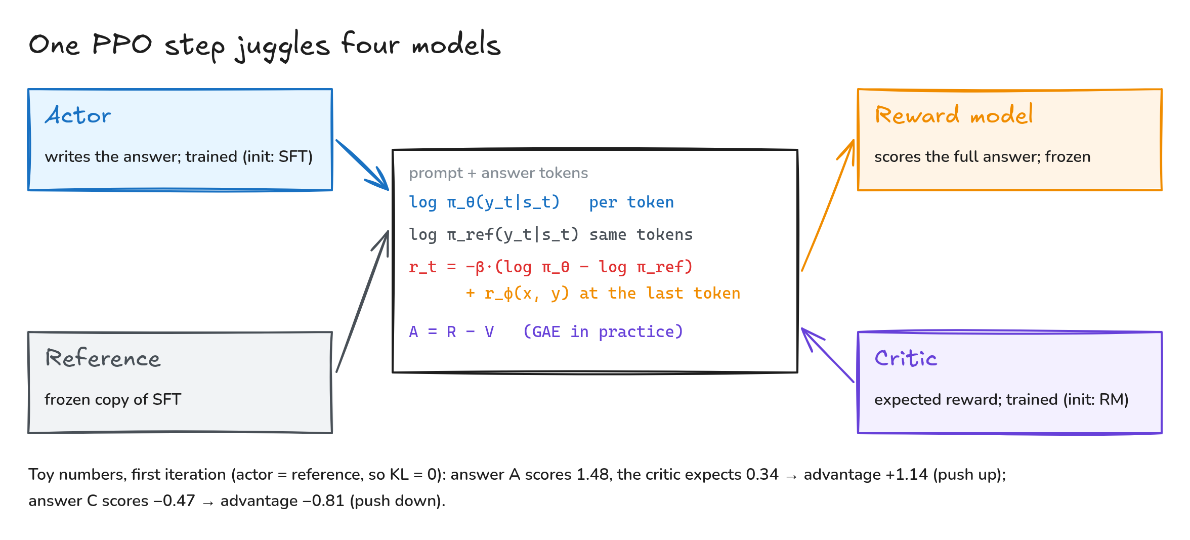
Fig. 5. Two models are trained (actor, critic) and two are frozen (reference, reward model).
- The actor \(\pi_\theta\) writes the answer and records each token’s log-probability. It starts as the SFT model and is trained.
- The reference \(\pi_{\text{ref}}\) is a frozen copy of the SFT model. It is fed the actor’s own prompt and answer and scores the very same tokens. The KL term compares the two models’ probabilities for identical text, which is why the reference reads the actor’s response instead of writing its own.
- The reward model \(r_\phi\) (frozen) grades the finished answer.
- The critic \(V_\psi\) (trained, initialized from the reward model) predicts how much reward to expect.
Per token, the reward is the KL penalty, plus the judge’s score on the last token:
\[r_t=-\beta\log\frac{\pi_\theta(y_t\mid s_t)}{\pi_{\text{ref}}(y_t\mid s_t)}\;+\;\begin{cases}r_\phi(x,y) & t=T\\0 & t<T\end{cases}\]The advantage asks whether this went better than the critic expected: \(A = R - V\). In practice it is computed per token with generalized advantage estimation (GAE), \(\delta_t=r_t+\gamma V(s_{t+1})-V(s_t)\) and \(A_t=\sum_{l\ge 0}(\gamma\lambda)^l\,\delta_{t+l}\). Subtracting the critic’s expectation is what makes the gradient far less noisy than the raw reward. In the toy run’s first iteration (actor = reference, so KL = 0), answer A scores 1.48 against an expected 0.34, an advantage of +1.14, so A is pushed up. Answer C gets −0.47 − 0.34 = −0.81, so it is pushed down.
PPO: small, safe steps
PPO (proximal policy optimization) compares the updated policy with the one that generated the data through a probability ratio, and then clips it:
\[\rho_t(\theta)=\frac{\pi_\theta(y_t\mid s_t)}{\pi_{\theta_{\text{old}}}(y_t\mid s_t)},\qquad L^{\text{CLIP}}(\theta)=\mathbb{E}_t\Big[\min\big(\rho_t A_t,\;\mathrm{clip}(\rho_t,1-\epsilon,1+\epsilon)\,A_t\big)\Big],\quad \epsilon=0.2\]Inside the band [0.8, 1.2] the update behaves like an ordinary policy gradient. Past the band the objective goes flat, so the gradient vanishes: a ratio of 1.35 on a good token counts only as 1.2. No single update can lurch too far.
This is what makes one batch of experience reusable, the point that confuses most people (it certainly confused me):
for iteration in 1, 2, 3, ...:
    prompts  = sample a batch of prompts                  # no reference answers needed
    answers  = actor.generate(prompts)                     # rollout, then FREEZE everything:
    store      log π_old, log π_ref, r_φ, V for every token
    compute    rewards r_t and advantages A_t once         # from the frozen batch
    for epoch in 1..K:                                      # K small, e.g. 4
        for minibatch in shuffle(batch):
            update actor with L_CLIP (ratio vs the frozen π_old)
            update critic toward the returns (MSE)
    discard the batch                                        # next iteration: fresh answers
The method is on-policy, but recycled a little. The ratio corrects for the drift between \(\pi_\theta\) and \(\pi_{\text{old}}\) during the \(K\) epochs, and the clip caps that drift.
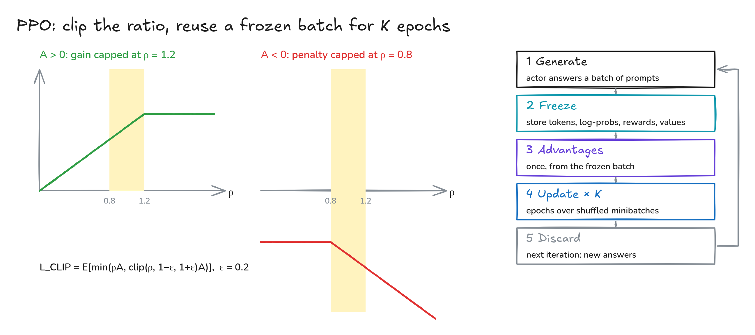
Fig. 6. Left: the clip caps the gain when A > 0 and the penalty when A < 0. Right: generate → freeze → compute advantages → K epochs of updates → discard.
7. A toy run you can check by hand
To see the dynamics without a GPU, shrink the policy to a distribution over our four answers. The SFT model starts at A 30%, B 35%, C 25%, D 10%. The judge’s scores are the reward model’s 1.48, 0.47, −0.47, −1.48. PPO runs with \(\beta = 1\), batch 256, \(K = 4\) epochs and \(\epsilon = 0.2\). Iteration by iteration, probability flows toward A. In the first iteration, 26% of the samples hit the clip. After 40 iterations the policy is A 64.0%, B 27.2%, C 7.5%, D 1.4%, the average reward has risen from 0.34 to 1.01, and the KL from the SFT model is 0.30.
That is no accident. The KL-regularized objective has a closed-form optimum. Maximize \(\sum_y \pi(y)\,r(y)-\beta\sum_y\pi(y)\log\frac{\pi(y)}{\pi_{\text{ref}}(y)}\) subject to \(\sum_y\pi(y)=1\), and setting the derivative to zero gives
\[\pi^{*}(y\mid x)=\frac{1}{Z(x)}\,\pi_{\text{ref}}(y\mid x)\,e^{\,r(x,y)/\beta}\]So the best policy is the SFT model, reweighted by \(e^{r/\beta}\). For our numbers it is 64.0%, 27.2%, 7.6%, 1.1%, which PPO reaches to within sampling noise. Now cut the leash and set \(\beta = 0\): the policy collapses onto one answer (A at 99%, KL 1.15). Here the judge happens to be right. If it had a blind spot, the policy would collapse onto that blind spot just as eagerly.
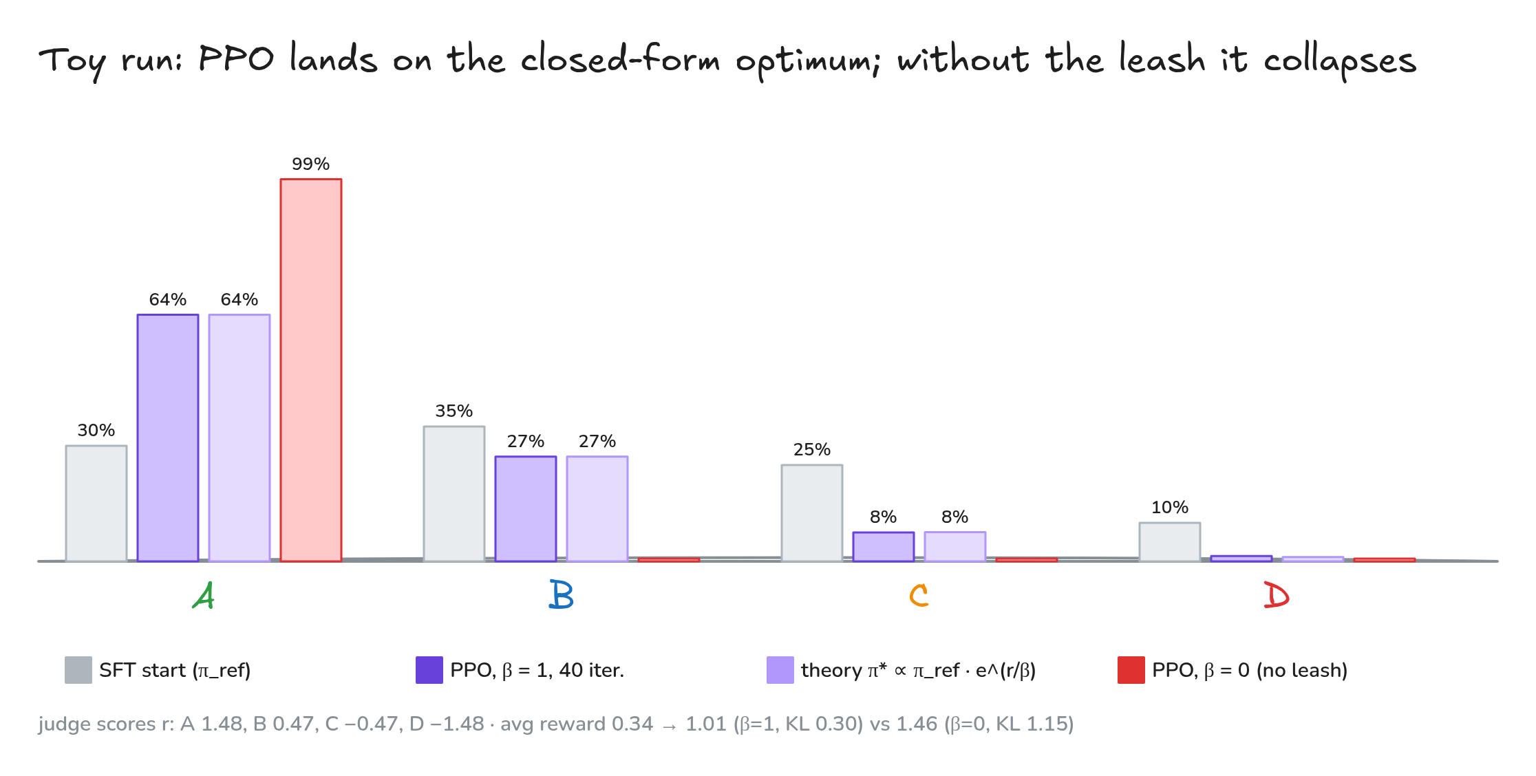
Fig. 7. PPO lands on π* ∝ π_ref·e^(r/β). Without the KL leash it collapses onto one answer.
8. Try it yourself (Python)
The whole toy pipeline in NumPy: a Bradley–Terry reward model fit to the ranking, PPO with clip, KL penalty and critic baseline, and the closed-form check. The output below is pasted from a real run (NumPy 2.4).
"""Toy RLHF in NumPy: one prompt, four candidate answers.
1) fit a Bradley-Terry reward model to one human ranking A > B > C > D,
2) run PPO (clipped ratio, KL penalty to the SFT policy, critic baseline),
3) check the result against the closed form  pi*(y) ∝ pi_ref(y) * exp(r(y)/beta)."""
import itertools
import numpy as np

sig = lambda z: 1 / (1 + np.exp(-z))
softmax = lambda z: np.exp(z - z.max()) / np.exp(z - z.max()).sum()

# ---- 1. reward model: one score per answer, pairwise loss -log sigma(r_w - r_l), L2 weight decay
pairs = list(itertools.combinations(range(4), 2))       # ranking A>B>C>D -> 6 (winner, loser) pairs
r, lam = np.zeros(4), 0.05
bt_loss = lambda r: np.mean([-np.log(sig(r[w] - r[l])) for w, l in pairs])
print(f"RM loss before: {bt_loss(r):.3f}")                 # ln 2: every pair is a coin flip
for step in range(4000):
    g = lam * r
    for w, l in pairs:
        d = sig(r[w] - r[l]) - 1                           # dL/dDelta
        g[w] += d / len(pairs); g[l] -= d / len(pairs)
    r -= 0.5 * g
r -= r.mean()                                              # only differences matter
print(f"RM loss after:  {bt_loss(r):.3f}   scores A..D = {np.round(r, 2)}")
d = r[0] - r[1]
print(f"A vs B: delta {d:.2f}, P(A>B) = {sig(d):.2f}, loss {-np.log(sig(d)):.2f}, flipped {-np.log(sig(-d)):.2f}")

# ---- 2. PPO on a policy over the four answers
ref = np.array([0.30, 0.35, 0.25, 0.10])                   # the SFT model = reference policy
def ppo(beta, iters=40, batch=256, mb=64, K=4, eps=0.2, lr=0.1, seed=7):
    rng = np.random.default_rng(seed)
    th, V = np.log(ref).copy(), float(ref @ r)             # actor logits; critic starts at E_ref[r]
    for it in range(iters):
        p_old = softmax(th)
        ys = rng.choice(4, size=batch, p=p_old)            # rollout (then frozen)
        R = r[ys] - beta * (np.log(p_old[ys]) - np.log(ref[ys]))   # judge score - KL penalty
        A = R - V                                          # advantage
        for _ in range(K):                                 # K epochs over the SAME batch
            idx = rng.permutation(batch)
            for s in range(0, batch, mb):
                b = idx[s:s + mb]; p = softmax(th); rho = p[ys[b]] / p_old[ys[b]]
                keep = rho * A[b] <= np.clip(rho, 1 - eps, 1 + eps) * A[b]   # min() picked the unclipped term
                g = np.zeros(4)
                for y, a, q in zip(ys[b][keep], A[b][keep], rho[keep]):
                    g -= a * q * (np.eye(4)[y] - p) / len(b)   # gradient of -rho*A w.r.t. logits
                th -= lr * g
                V += 0.5 * np.mean(R[b] - V)               # critic regresses toward the returns
    return softmax(th)

pi = ppo(beta=1.0)
star = ref * np.exp(r / 1.0); star /= star.sum()
kl = lambda p: np.sum(p * np.log(np.clip(p, 1e-12, 1) / ref))
V0 = round(float(ref @ r), 2)                              # critic expectation at iteration 1 (KL = 0 there)
print(f"advantage at iteration 1 (V = {V0}): A {round(r[0], 2) - V0:+.2f}, C {round(r[2], 2) - V0:+.2f}")
print("PPO  beta=1:", np.round(pi, 3), f"avg reward {pi @ r:.2f}, KL {kl(pi):.2f}")
print("closed form:", np.round(star, 3))
pi0 = ppo(beta=0.0)
print("PPO  beta=0:", np.round(pi0, 3), f"avg reward {pi0 @ r:.2f}, KL {kl(pi0):.2f}")

# RM loss before: 0.693
# RM loss after:  0.212   scores A..D = [ 1.48  0.47 -0.47 -1.48]
# A vs B: delta 1.01, P(A>B) = 0.73, loss 0.31, flipped 1.32
# advantage at iteration 1 (V = 0.34): A +1.14, C -0.81
# PPO  beta=1: [0.64  0.272 0.075 0.014] avg reward 1.01, KL 0.30
# closed form: [0.64  0.272 0.076 0.011]
# PPO  beta=0: [0.992 0.005 0.002 0.001] avg reward 1.46, KL 1.15
In a real LLM the “four answers” become all possible token sequences, the scores come from a 6B reward model, and the gradient flows per token through the Transformer, but the loop is the same.
9. Did it work?
| InstructGPT result (Ouyang et al. 2022) | |
|---|---|
| Preference | Labelers preferred the 1.3B InstructGPT model over the 175B GPT-3, 100× smaller |
| Head to head at 175B | InstructGPT outputs preferred 85 ± 3% of the time |
| Made-up facts (closed-domain tasks) | 41% → 21% |
| Toxicity, when prompted to be respectful | about 25% fewer toxic outputs |
| Cost of alignment | SFT 4.9 + PPO-ptx 60 petaflop/s-days vs 3,640 for GPT-3 pretraining: about 1.8% |
Later in 2022 the same recipe, applied to conversations, became ChatGPT.
10. What came next
- DPO (Rafailov et al. 2023) rearranges the closed form above. Since \(r=\beta\log\frac{\pi^*}{\pi_{\text{ref}}}+\beta\log Z\), plug that into the Bradley–Terry loss. \(Z\) cancels, and the policy becomes its own reward model, trained directly on preference pairs with no separate reward model and no PPO: \(\mathcal{L}_{\text{DPO}}=-\log\sigma\Big(\beta\log\frac{\pi_\theta(y_w\mid x)}{\pi_{\text{ref}}(y_w\mid x)}-\beta\log\frac{\pi_\theta(y_l\mid x)}{\pi_{\text{ref}}(y_l\mid x)}\Big)\)
- GRPO (Shao et al. 2024; used for DeepSeek’s reasoning models) drops the critic. It samples a group of \(G\) answers per prompt and uses the group as the baseline, \(A_i=\frac{r_i-\mathrm{mean}(r_1,\dots,r_G)}{\mathrm{std}(r_1,\dots,r_G)}\). With our four scores (and the population standard deviation) this gives +1.35, +0.43, −0.43, −1.35.
- Verifiable rewards. For math and code, the judge can simply be a checker that verifies the answer or runs the unit tests.
Myths and truths
| Myth | Truth |
|---|---|
| Humans give each answer a score. | They rank answers. The reward model turns rankings into numbers through pairwise comparisons. |
| The reward model knows what’s true. | It learned what labelers prefer. That usually tracks truth, not always, and a policy can exploit the gap (reward hacking). |
| PPO needs correct reference answers. | It needs only prompts (~31,000 in InstructGPT). The reward model does the grading. |
| RLHF teaches the model new knowledge. | Knowledge comes mostly from pretraining. RLHF, at about 2% of the compute, shapes how that knowledge is used. |
| PPO reuses data, so it is off-policy. | It is on-policy but recycled for \(K\) epochs. The ratio and the clip keep the reuse safe, then the batch is discarded. |
Cheat sheet
| Term | Meaning |
|---|---|
| Token | a piece of text; GPT-3 has 50,257 of them |
| Pretraining | next-token cross-entropy on internet text |
| SFT | the same loss on human-written answers (answer tokens only) |
| Reward model \(r_\phi\) | SFT Transformer + scalar head, trained with \(-\log\sigma(r_w-r_l)\) |
| Policy / actor \(\pi_\theta\) | the language model being optimized |
| Reference \(\pi_{\text{ref}}\) | a frozen SFT copy, the anchor of the KL leash |
| Critic \(V_\psi\) | predicts the expected reward, giving a baseline for the advantage |
| Advantage \(A\) | reward − expectation: better or worse than expected? |
| Ratio \(\rho\), clip \(\epsilon\) | new/old probability; kept within \(1\pm0.2\) |
| \(\beta\) | leash strength; \(\beta\to0\) invites collapse and reward hacking |
| \(\pi^*\propto\pi_{\text{ref}}e^{r/\beta}\) | the optimum PPO is chasing; the basis of DPO |
Papers: Brown et al. 2020 (GPT-3), Ouyang et al. 2022 (InstructGPT), Christiano et al. 2017 and Stiennon et al. 2020 (learning from human preferences), Schulman et al. 2017 (PPO) and 2016 (GAE), Rafailov et al. 2023 (DPO), Shao et al. 2024 (GRPO). The next-token probabilities, the four answers, the per-token log-probabilities in the video and the GRPO bars are illustrative; the reward-model scores and the PPO run are a real toy computation (section 8). Tokens are from the GPT-3 tokenizer (r50k_base). Figures were drawn with Excalidraw; the editable sources open directly on excalidraw.com: Fig. 1, Fig. 2, Fig. 3, Fig. 4, Fig. 5, Fig. 6, Fig. 7. The video was animated with Remotion and narrated with a synthetic (text-to-speech) voice, Kokoro-82M. The music is an original ambient score generated procedurally for this video (no license needed).