What is a Transformer? A visual guide, told with one T-cell receptor

In one sentence: a Transformer turns a sequence into vectors and, layer by layer, lets every token gather information from every other token through attention, then refines each token with a small neural network.
\[\mathrm{Attention}(Q,K,V)=\mathrm{softmax}\!\left(\frac{QK^{\top}}{\sqrt{d_k}}\right)V\]

The video above and the walkthrough below share one running example, thirteen letters long, CASSIRSSYEQYF: the CDR3β loop of a public T-cell receptor that recognizes the influenza peptide GILGFVFTL on HLA-A*02:01 and turns up in many people. The toy numbers come from a tiny hand-built model you can run yourself (section 8). The ESM-2 numbers come from a real protein language model.

1. The problem: every letter needs context

The letter S appears four times in CASSIRSSYEQYF, but each S sits among different neighbors (A·S·S, S·S·I, R·S·S, S·S·Y), so each plays a slightly different role. A model has to read every letter in context.

Recurrent networks (RNNs) read one letter at a time and pass a running memory down the line. That is slow, because step 13 has to wait for step 12, and forgetful, because by the end the first letters have faded. In 2017, Attention Is All You Need (Vaswani et al.) proposed the fix: connect every letter to every other letter directly, and process them all in parallel.

2. Letters become vectors that know their position

Each amino acid becomes a token, and each token becomes a vector, a short list of numbers. Real models learn these numbers (ESM-2 650M uses 1,280 per residue). Our toy uses four that a chemist would recognize: hydropathy (Kyte–Doolittle ÷ 4.5), charge, polarity and aromaticity.

Attention on its own treats a sequence like a bag of letters: shuffle the input and the outputs are merely shuffled too. So we add a positional encoding made of sine and cosine waves of different frequencies:

\[PE_{(pos,\,2i)}=\sin\!\left(\frac{pos}{10000^{2i/d}}\right)\qquad PE_{(pos,\,2i+1)}=\cos\!\left(\frac{pos}{10000^{2i/d}}\right)\]

Real models add this to the token vector. For readability our toy stacks them: 4 chemistry numbers plus 4 position numbers (base 9 instead of 10000, two frequencies) gives 8 numbers per residue.

Fig. 1. The toy input: one 8-number vector per residue

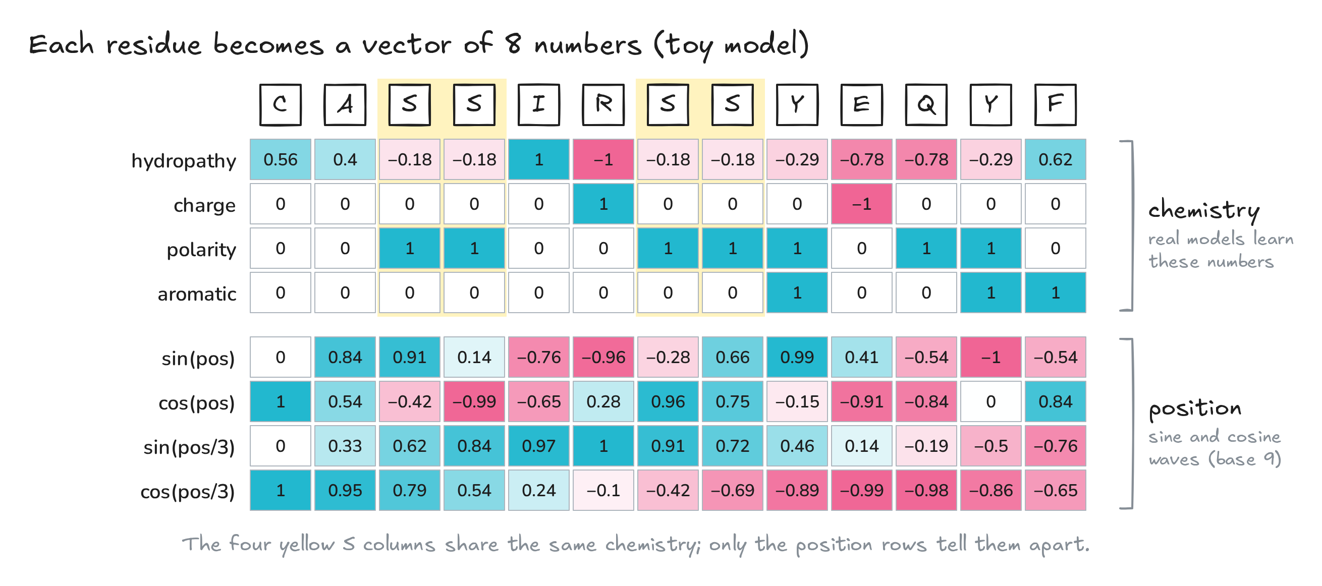
Fig. 1. The toy input: one 8-number vector per residue

3. Query, key, value

From its vector \(\mathbf{x}\), every residue makes three new vectors with three learned matrices:

\[\mathbf{q}=\mathbf{x}W_Q \qquad \mathbf{k}=\mathbf{x}W_K \qquad \mathbf{v}=\mathbf{x}W_V\]

The query asks “what am I looking for?”, the key says “what do I offer?”, and the value is what the residue passes on if someone listens. In our first head, arginine’s query says: I’m looking for a negative partner. How well a query matches a key is their dot product, which measures alignment.

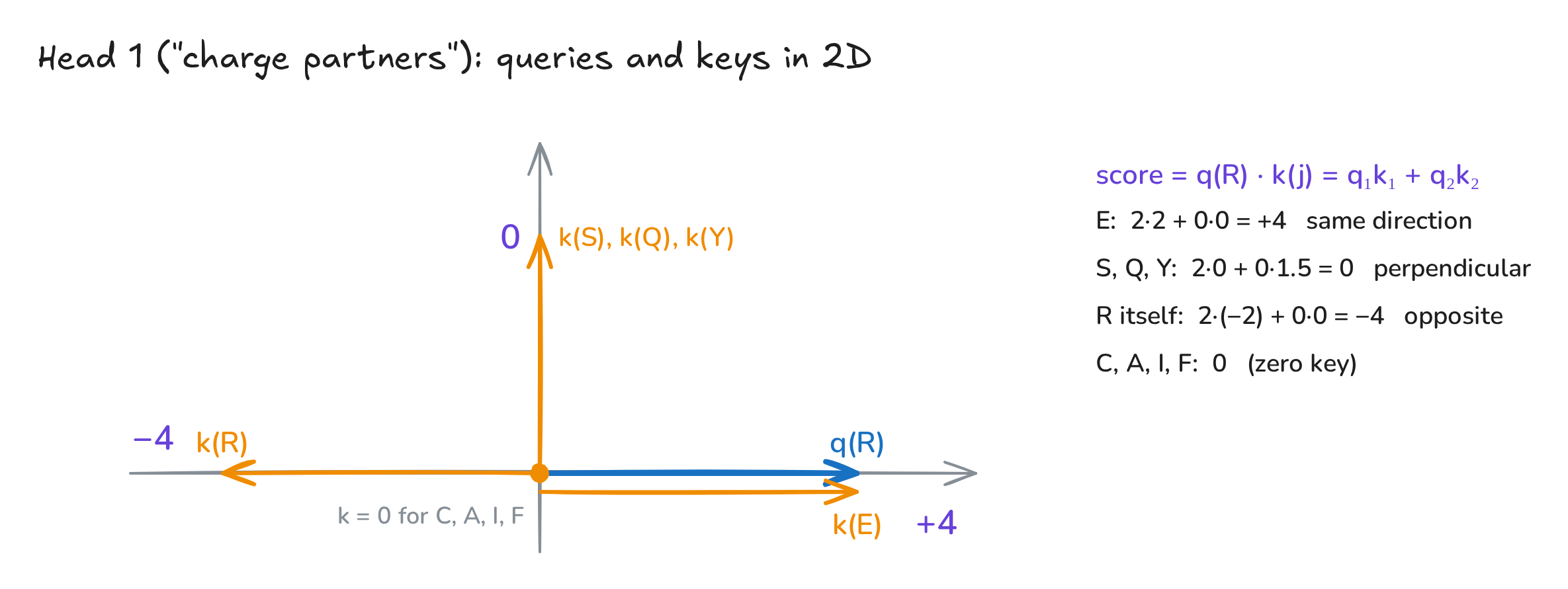
Fig. 2. Dot products in a two-dimensional head

Fig. 2. Dot products in a two-dimensional head

4. The attention formula, one step at a time

\[\mathrm{Attention}(Q,K,V)=\mathrm{softmax}\!\left(\frac{QK^{\top}}{\sqrt{d_k}}\right)V\]

Follow arginine (R, position 6) through one head:

Score its query against every key: glutamate +4, arginine itself −4, everyone else 0.
Scale by \(\sqrt{d_k}=\sqrt{2}\): +2.83, −2.83 and 0.
Softmax turns scores into positive weights that add up to one, \(a_j=e^{s_j}/\sum_k e^{s_k}\). Glutamate gets 0.605, each of the other eleven residues 0.036, arginine 0.002. By hand: \(e^{2\sqrt2}/(e^{2\sqrt2}+11+e^{-2\sqrt2})=0.605\).
Blend the values with those weights: \(\mathbf{z}_R=\sum_j a_{Rj}\,\mathbf{v}_j=[-0.60,\ 0.25]\). Arginine’s new vector now carries news from glutamate.

Fig. 3. Arginine's row of attention

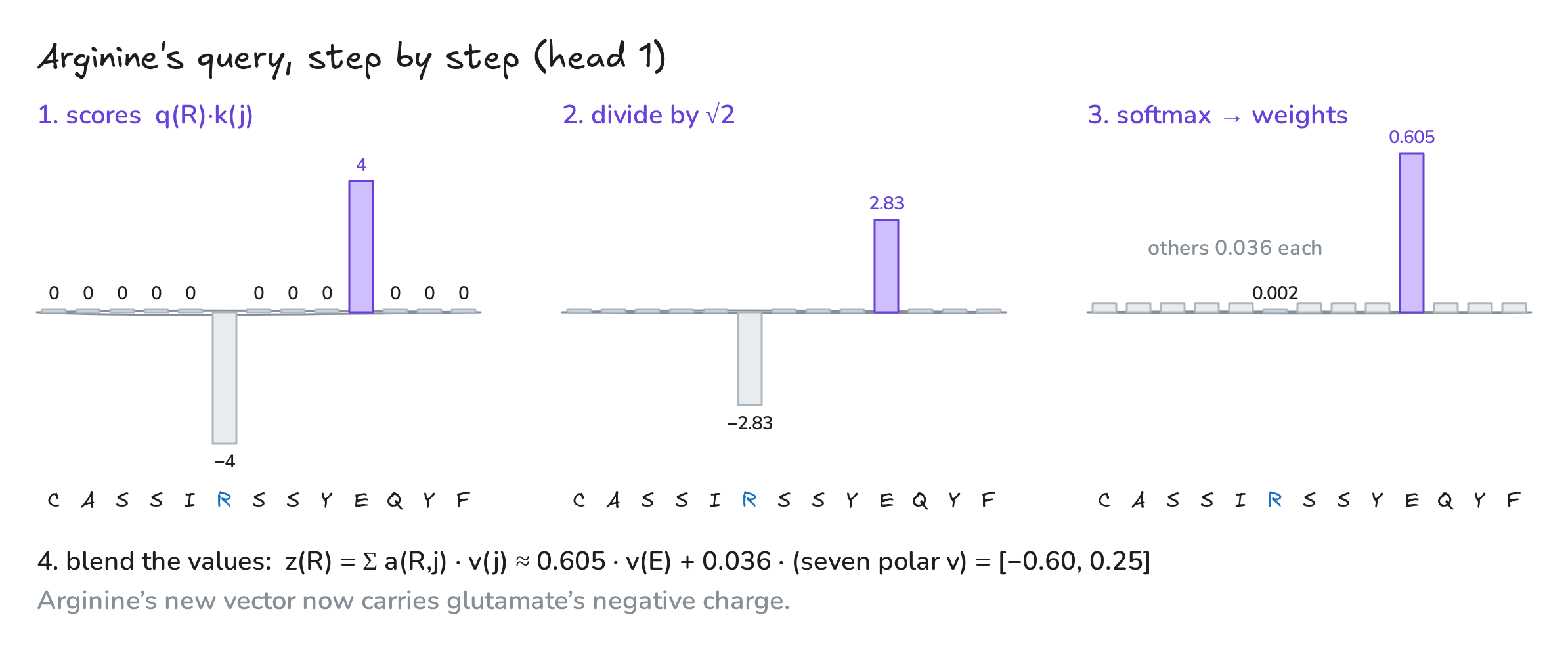
Fig. 3. Arginine’s row of attention

Why divide by \(\sqrt{d_k}\)? In ESM-2 each query and key has \(d_k=64\) numbers, and dot products grow with dimension. With 13 random 64-number keys, the raw scores spread by about ±6, softmax turns spiky (one key takes 99.8% of the weight) and learning stalls because the gradients vanish. Dividing by \(\sqrt{64}=8\) keeps the weights spread out (the largest is 33%).

5. The attention map and many heads

Every residue does this at the same time. With the queries stacked into \(Q\) and the keys into \(K\), a single matrix product \(QK^{\top}\) gives all \(13\times13=169\) scores, which is why Transformers train so fast on GPUs. After a softmax on each row, row \(i\) of the attention map shows where residue \(i\) looks. The price is that the number of pairs grows with the square of the length: a 1,000-residue protein means a million pairs per head, per layer.

One head captures only one kind of relationship, so Transformers run several heads in parallel, each with its own \(W_Q\), \(W_K\) and \(W_V\), then join their outputs side by side and mix them with one more matrix:

\[\mathrm{MultiHead}(X)=\mathrm{Concat}(\mathrm{head}_1,\dots,\mathrm{head}_h)\,W_O\]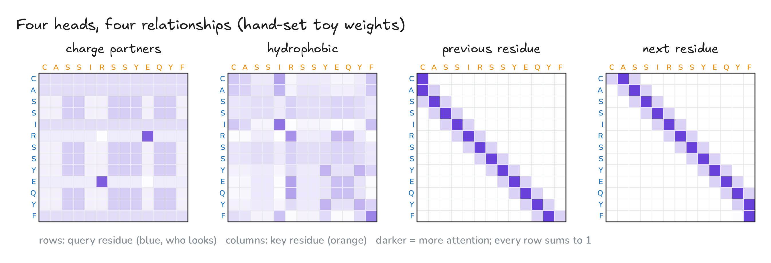

Fig. 4. The four heads of the toy model

Fig. 4. The four heads of the toy model

In our toy, one head pairs charges, one links hydrophobic residues, one looks at the previous residue and one at the next. The four S’s entered with identical chemistry and leave as four different vectors, because the last two heads pulled in their different neighbors.

6. The Transformer block

Attention is only half of a block. The other half is a small feed-forward network applied to each residue on its own: expand, apply a nonlinearity, compress.

\[\mathrm{FFN}(\mathbf{x})=W_2\,\mathrm{GELU}(W_1\mathbf{x}+b_1)+b_2\]

An easy way to remember it: attention lets residues talk to each other, the feed-forward network lets each one think. Around each half runs a residual connection (a shortcut that adds the input back), plus layer normalization to keep the numbers stable:

\[\mathbf{x}\leftarrow\mathbf{x}+\mathrm{MHA}(\mathrm{LN}(\mathbf{x}))\qquad\mathbf{x}\leftarrow\mathbf{x}+\mathrm{FFN}(\mathrm{LN}(\mathbf{x}))\]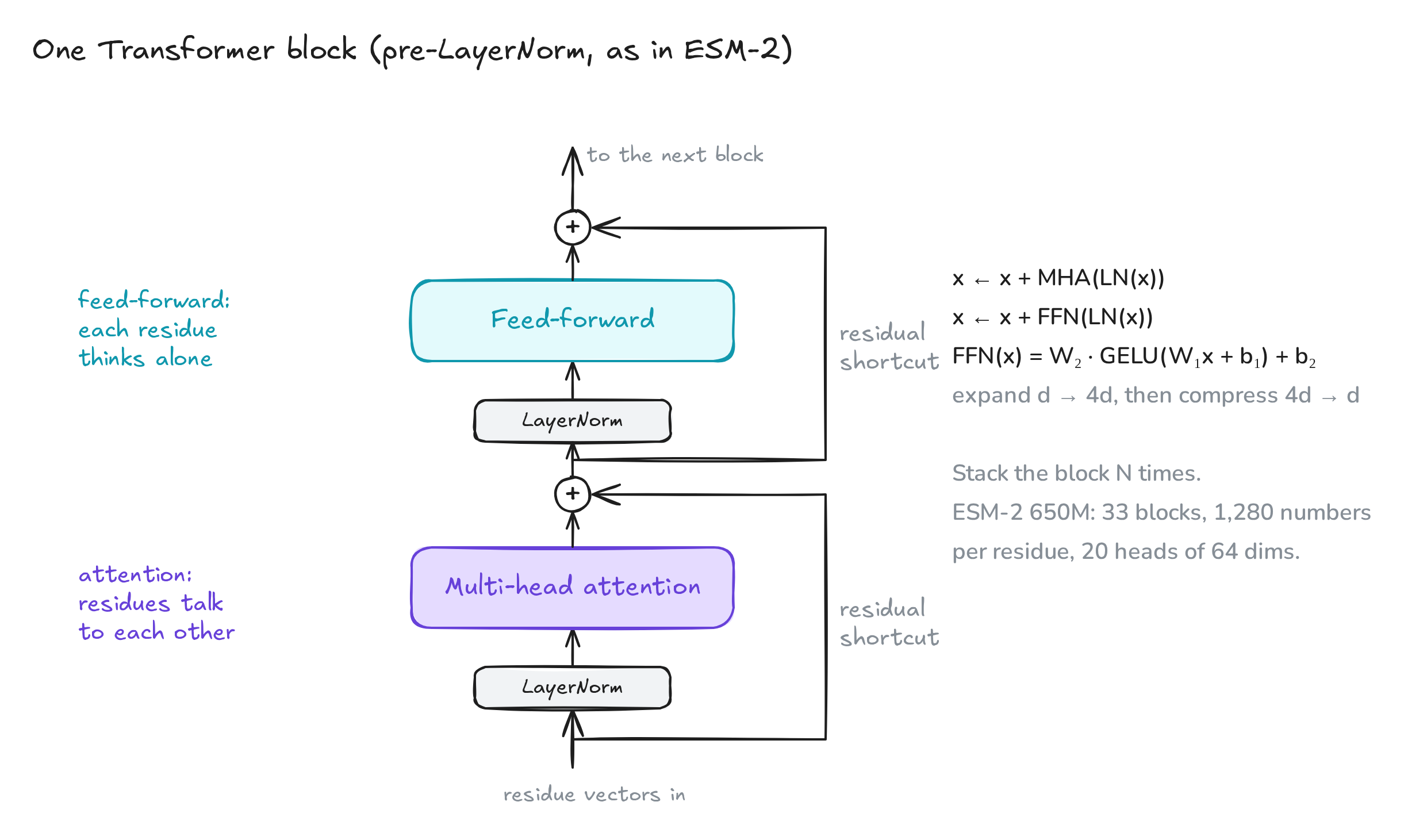

Fig. 5. One pre-LayerNorm Transformer block

Fig. 5. One pre-LayerNorm Transformer block

Then you stack blocks: ESM-2 650M stacks 33 of them, with 1,280 numbers per residue and 20 heads.

7. Three family members, and how they learn

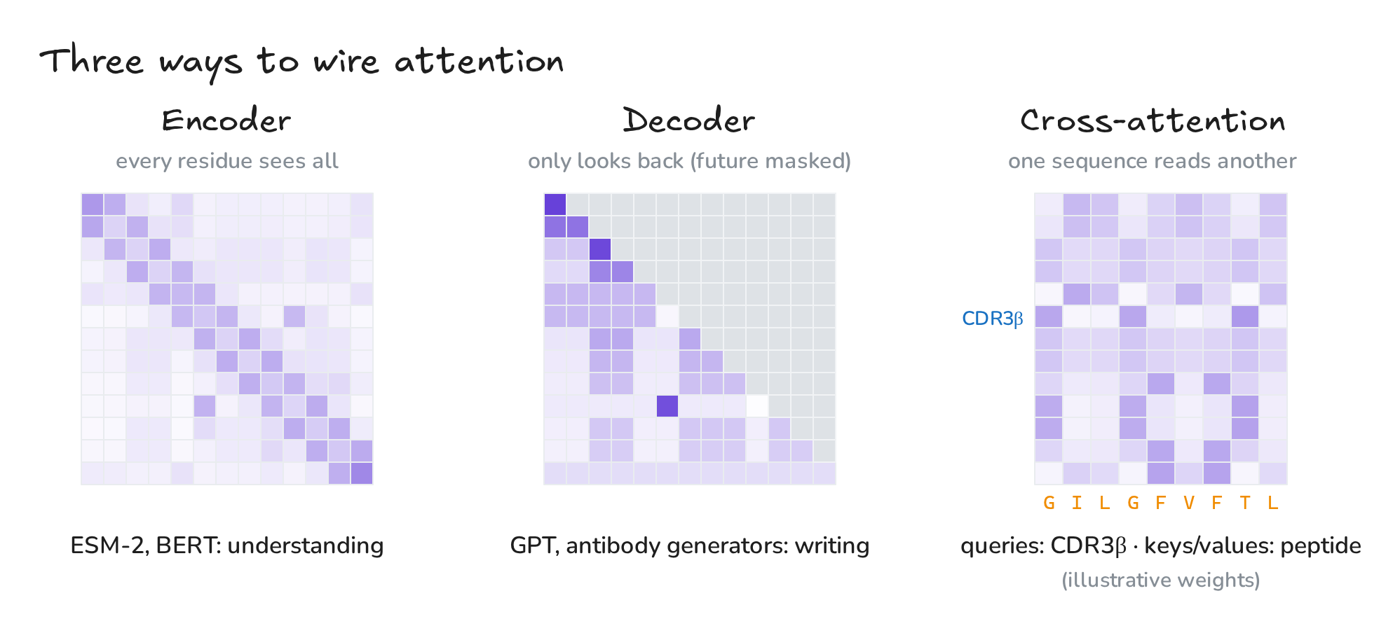
Fig. 6. Encoder, decoder and cross-attention

Fig. 6. Encoder, decoder and cross-attention

An encoder lets every residue see the whole sequence; ESM-2 and BERT are encoders, built for understanding. A decoder masks the future so that each position can only look back,

\[\mathrm{softmax}\!\left(\frac{QK^{\top}}{\sqrt{d_k}}+M\right)V,\qquad M_{ij}=\begin{cases}0 & j\le i\\ -\infty & j>i\end{cases}\]

which lets it write new sequences one residue at a time, like GPT or generative antibody models. Cross-attention connects two sequences: queries from the T-cell receptor, keys and values from the peptide.

How does a protein model learn? With a simple game: hide a residue and guess it. Training minimizes

\[\mathcal{L}=-\log p_\theta(\text{true residue}\mid\text{rest of chain})\]

and backpropagation nudges every weight to do better, across millions of proteins. Here is a real, small model (ESM-2 with 12 layers) reading the whole 131-residue TCRβ chain:

Fig. 7. ESM-2 guesses a hidden residue

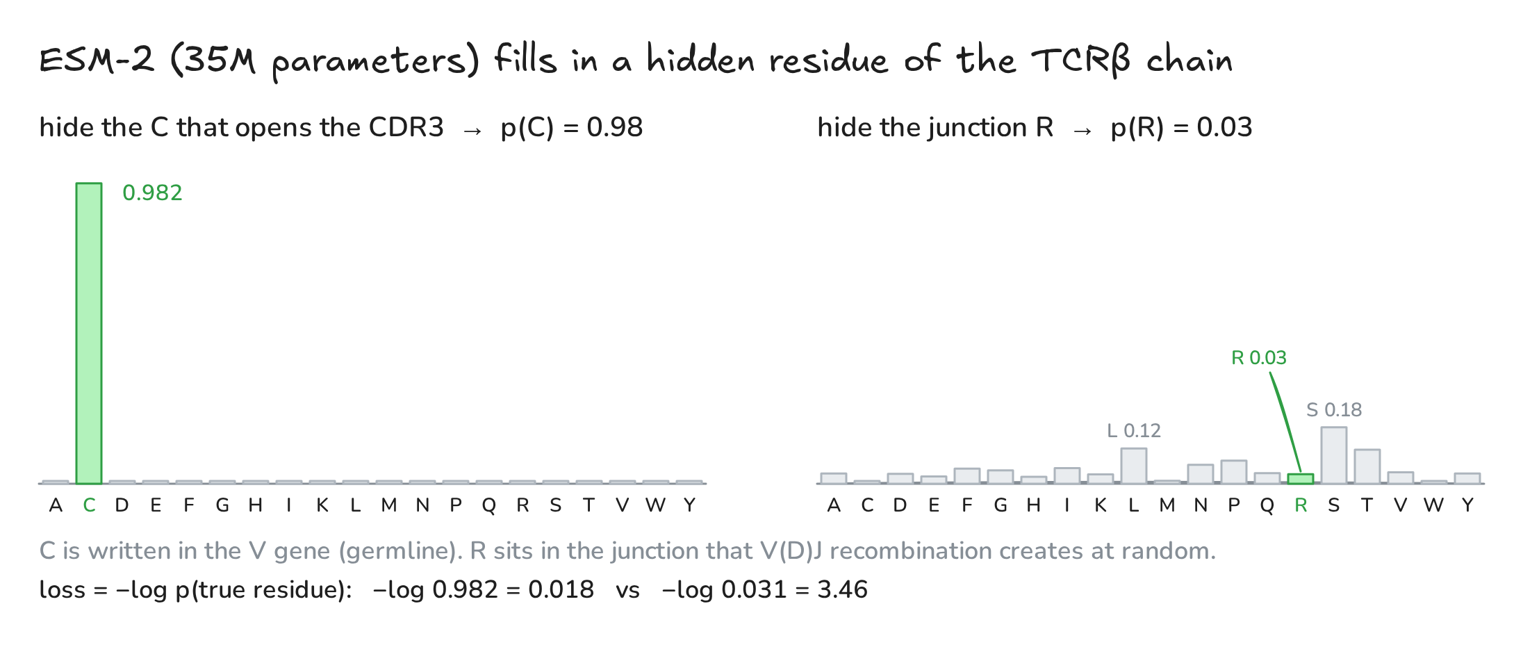
Fig. 7. ESM-2 guesses a hidden residue

It is 98% sure about the cysteine that opens the CDR3 but gives only 3% to the arginine. That is biology, not failure: the cysteine is written in the V gene, while the arginine sits in the junction that V(D)J recombination creates at random.

8. Build it in NumPy

Here is everything above in about 100 lines of NumPy: the toy input, attention, four heads, multi-head attention, one full block, and a check against PyTorch’s own TransformerEncoderLayer.

"""A Transformer, hand-built in NumPy, reading a T-cell receptor CDR3β.
Companion code for the video "What is a Transformer?". Toy model: 8 numbers per residue,
4 hand-set attention heads (d_k = 2). Only NumPy is required; PyTorch is used for an optional check."""
import numpy as np
from math import erf

# 1. Tokens -> vectors ------------------------------------------------------------------
SEQ = "CASSIRSSYEQYF"   # CDR3β of a public flu-specific TCR (binds GILGFVFTL on HLA-A*02:01)
KD = dict(A=1.8, C=2.5, E=-3.5, F=2.8, I=4.5, Q=-3.5, R=-4.5, S=-0.8, Y=-1.3)  # Kyte-Doolittle
CHARGED, POLAR, AROMATIC = dict(R=1, K=1, D=-1, E=-1), set("STNQYH"), set("FWY")

def embed(a):  # 4 "chemistry" numbers per residue; real models learn these instead
    return [round(KD[a] / 4.5, 2), CHARGED.get(a, 0), float(a in POLAR), float(a in AROMATIC)]

def pos_enc(n, d=4, base=9.0):  # sinusoidal positions (the paper uses base 10000, d = d_model)
    pos, i = np.arange(n)[:, None], np.arange(d // 2)[None, :]
    ang = pos / base ** (2 * i / d)
    P = np.zeros((n, d))
    P[:, 0::2], P[:, 1::2] = np.sin(ang), np.cos(ang)
    return P

X = np.hstack([np.array([embed(a) for a in SEQ], float), pos_enc(len(SEQ))])  # 13 x 8

# 2. Attention ---------------------------------------------------------------------------
def softmax(S):
    E = np.exp(S - S.max(-1, keepdims=True))
    return E / E.sum(-1, keepdims=True)

def attention(X, Wq, Wk, Wv):
    Q, K, V = X @ Wq, X @ Wk, X @ Wv       # 1 project
    S = Q @ K.T / np.sqrt(K.shape[-1])     # 2 score every pair, then scale
    A = softmax(S)                         # 3 each row sums to 1
    return A @ V, A                        # 4 blend the values

# 3. Four hand-set heads, d_k = 2 -------------------------------------------------------
HYD, CHG, POL, ARO, P1s, P1c, P2s, P2c = range(8)      # meaning of the 8 input numbers
W = [{m: np.zeros((8, 2)) for m in "QKV"} for _ in range(4)]
W[0]["Q"][CHG, 0], W[0]["Q"][POL, 1] = 2.0, 1.5       # head 1: + looks for -, polar for polar
W[0]["K"][CHG, 0], W[0]["K"][POL, 1] = -2.0, 1.5
W[0]["V"][CHG, 0], W[0]["V"][POL, 1] = 1.0, 1.0
W[1]["Q"][HYD, 0], W[1]["Q"][ARO, 1] = 2.0, 1.5       # head 2: hydrophobic finds hydrophobic
W[1]["K"][HYD, 0], W[1]["K"][ARO, 1] = 2.0, 1.5
W[1]["V"][HYD, 0], W[1]["V"][ARO, 1] = 1.0, 1.0
w, s = 1 / 3, 50.0                                     # heads 3-4: previous / next residue,
for h, d in [(2, -1), (3, +1)]:                        # by rotating the slow position wave
    W[h]["Q"][P2s, 0], W[h]["Q"][P2c, 0] = s * np.cos(w), s * d * np.sin(w)
    W[h]["Q"][P2s, 1], W[h]["Q"][P2c, 1] = -s * d * np.sin(w), s * np.cos(w)
    W[h]["K"][P2s, 0], W[h]["K"][P2c, 1] = 1.0, 1.0
    W[h]["V"][HYD, 0], W[h]["V"][CHG, 1] = 1.0, 1.0

Z, A = attention(X, W[0]["Q"], W[0]["K"], W[0]["V"])
print("head 1, row R:", A[5].round(3))
print("R -> E weight:", A[5, 9].round(3), "  z_R =", Z[5].round(3))

# 4. Multi-head attention ------------------------------------------------------------------
def multi_head(X, W, Wo):
    outs = [attention(X, w["Q"], w["K"], w["V"]) for w in W]
    return np.hstack([z for z, _ in outs]) @ Wo, [a for _, a in outs]

ctx, maps = multi_head(X, W, np.eye(8))
for i in [2, 3, 6, 7]:
    print(f"S at {i + 1:>2}: before {X[i, :4]}  after {ctx[i].round(2)}")

# 5. One full Transformer block (pre-LayerNorm, as in ESM-2) -------------------------------
def layer_norm(x, eps=1e-5):
    return (x - x.mean(-1, keepdims=True)) / np.sqrt(x.var(-1, keepdims=True) + eps)

def gelu(x):
    return 0.5 * x * (1 + np.vectorize(erf)(x / np.sqrt(2)))

rng = np.random.default_rng(0)
Wo = rng.normal(0, 0.3, (8, 8))                        # mixes the 4 heads
W1, b1 = rng.normal(0, 0.3, (8, 32)), np.zeros(32)     # expand d -> 4d
W2, b2 = rng.normal(0, 0.3, (32, 8)), np.zeros(8)      # compress 4d -> d

def block(x):
    x = x + multi_head(layer_norm(x), W, Wo)[0]              # residues talk (attention)
    return x + gelu(layer_norm(x) @ W1 + b1) @ W2 + b2       # each residue thinks (FFN)

Y = block(X)
print("block output:", Y.shape, " attention params:", 4 * 8 * 8, " FFN params:", 2 * 8 * 32)

# 6. Check against PyTorch's own layer ---------------------------------------------------
try:
    import torch, torch.nn as nn
    layer = nn.TransformerEncoderLayer(d_model=8, nhead=4, dim_feedforward=32, dropout=0.0,
                                       activation="gelu", norm_first=True, batch_first=True)
    cat = lambda m: np.hstack([w[m] for w in W]).T          # PyTorch stores (out, in)
    t = lambda a: torch.tensor(a, dtype=torch.float32)
    with torch.no_grad():
        layer.self_attn.in_proj_weight.copy_(t(np.vstack([cat("Q"), cat("K"), cat("V")])))
        layer.self_attn.in_proj_bias.zero_()
        layer.self_attn.out_proj.weight.copy_(t(Wo.T)); layer.self_attn.out_proj.bias.zero_()
        layer.linear1.weight.copy_(t(W1.T)); layer.linear1.bias.zero_()
        layer.linear2.weight.copy_(t(W2.T)); layer.linear2.bias.zero_()
        Yt = layer(t(X[None]))[0].numpy()
    print("max |NumPy - PyTorch| =", f"{np.abs(Y - Yt).max():.1e}")
except ImportError:
    print("PyTorch not installed: skipping the check")

Output:

head 1, row R: [0.036 0.036 0.036 0.036 0.036 0.002 0.036 0.036 0.036 0.605 0.036 0.036
 0.036]
R -> E weight: 0.605   z_R = [-0.603  0.25 ]
S at  3: before [-0.18  0.    1.    0.  ]  after [ 0.    0.85 -0.26  0.21  0.35  0.   -0.05  0.  ]
S at  4: before [-0.18  0.    1.    0.  ]  after [ 0.    0.85 -0.26  0.21 -0.11  0.    0.65  0.11]
S at  7: before [-0.18  0.    1.    0.  ]  after [ 0.    0.85 -0.26  0.21 -0.69  0.78 -0.19  0.  ]
S at  8: before [-0.18  0.    1.    0.  ]  after [ 0.    0.85 -0.26  0.21 -0.27  0.11 -0.33 -0.11]
block output: (13, 8)  attention params: 256  FFN params: 512
max |NumPy - PyTorch| = 4.1e-06

Every number matches the figures, and the NumPy block agrees with PyTorch to about \(10^{-6}\) (float32 rounding). To reproduce the ESM-2 guesses (pip install fair-esm torch; downloads the 35M model once):

"""Hide one residue of a TCR beta chain and let ESM-2 guess it (pip install fair-esm torch)."""
import torch, esm

model, alphabet = esm.pretrained.esm2_t12_35M_UR50D()      # 12 layers, 35M parameters
model.eval()
V_GENE = ("MSNQVLCCVVLCLLGANTVDGGITQSPKYLFRKEGQNVTLSCEQNLNHDAMYWYRQDPGQGLRLIYY"
          "SQIVNDFQKGDIAEGYSVSREKKESFPLTVTSAQKNPTAFYL")    # TRBV19, up to the CDR3
CDR3, J_END = "CASSIRSSYEQYF", "GPGTRLTVT"                  # CDR3β, then the rest of TRBJ2-7
chain = V_GENE + CDR3 + J_END                               # 131 residues
AA = "ACDEFGHIKLMNPQRSTVWY"

def guess(k):  # mask CDR3 position k (0-based) and return p(amino acid) over the 20 residues
    tokens = alphabet.get_batch_converter()([("tcr", chain)])[2]
    i = len(V_GENE) + k + 1                                  # +1 for the <cls> token
    tokens[0, i] = alphabet.mask_idx
    with torch.no_grad():
        logits = model(tokens)["logits"][0, i]
    p = torch.softmax(logits[[alphabet.get_idx(a) for a in AA]], -1)
    return dict(zip(AA, p.tolist()))

for k in [0, 5]:
    p = guess(k); true = CDR3[k]
    top = sorted(p, key=p.get, reverse=True)[:4]
    print(f"hide {true}: p({true}) = {p[true]:.3f}   top: " + ", ".join(f"{a} {p[a]:.2f}" for a in top))

hide C: p(C) = 0.982   top: C 0.98, S 0.00, F 0.00, V 0.00
hide R: p(R) = 0.031   top: S 0.18, L 0.12, T 0.11, P 0.08

9. In the lab, and four traps

In immunology and drug discovery, the most common use is as a feature extractor: feed a TCR or antibody sequence into a pretrained protein language model, take one context-rich vector per residue, pool them, and train a small classifier to predict binding, specificity or developability. Antibody language models such as AntiBERTy and AbLang do the same for B-cell receptors, and AlphaFold uses attention to reason about pairs of residues in 3D.

Myth	Truth
Attention weights show which residues matter.	They show where information flowed, in one head. Importance needs ablations and experiments.
A Transformer knows the order of a sequence.	Only through positional encoding. Without it, it sees a bag of letters.
Most of the weights are in attention.	About two thirds sit in the feed-forward layers: per block, attention has \(4d^2\) weights and the FFN \(8d^2\).
Transformers are just for language.	They work on any sequence of tokens: amino acids, nucleotides, even cells.

10. My study notes: the full Transformer in PyTorch

Sections 1–9 follow one block through one receptor. These are the notes I wrote while studying the whole architecture: the original encoder–decoder from Attention Is All You Need (Vaswani et al., 2017), rebuilt module by module in PyTorch, with the shapes and the “why” for each part. Two details differ from the ESM-2 block in Section 6, on purpose: the paper puts LayerNorm after each residual addition (Post-LN), and its feed-forward network uses ReLU instead of GELU.

The complete code, with every output, is also available as a notebook: transformer-pytorch.ipynb (needs only torch).

10.1 The parts list

Module	What it does	Shape in → out
Embedding + positional encoding	Turns token IDs into vectors and stamps each one with its position	`(B, L)` → `(B, L, d_model)`
Multi-head attention	Lets every position gather information from the others, through several heads at once	`(B, L, d_model)` → `(B, L, d_model)`
Position-wise feed-forward	Two linear layers applied to each position on its own	`(B, L, d_model)` → `(B, L, d_ff)` → `(B, L, d_model)`
Add & Norm	Residual shortcut plus LayerNorm around every sub-layer	shape unchanged
Encoder layer	Self-attention, then feed-forward	shape unchanged
Decoder layer	Masked self-attention, cross-attention to the encoder, then feed-forward	shape unchanged
Output projection	One linear layer to scores over the vocabulary	`(B, L, d_model)` → `(B, L, vocab)`

Here B is the batch size and L the sequence length. The paper’s base model uses \(d_{model}=512\), 8 heads, \(d_{ff}=2048\) and 6 layers in each stack.

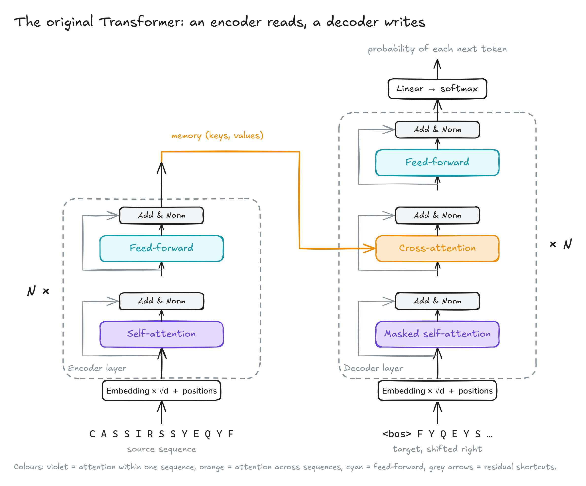
Fig. 8. The whole encoder–decoder. Each dashed box is one layer, repeated N times; the encoder's output feeds every decoder layer through cross-attention

Fig. 8. The whole encoder–decoder. Each dashed box is one layer, repeated N times; the encoder’s output feeds every decoder layer through cross-attention

10.2 Positional encoding

Attention by itself is blind to order: shuffle the residues and every output is shuffled the same way. The original Transformer adds a fixed pattern of sines and cosines to each embedding:

\[PE_{(pos,\,2i)}=\sin\!\left(\frac{pos}{10000^{2i/d_{model}}}\right)\qquad PE_{(pos,\,2i+1)}=\cos\!\left(\frac{pos}{10000^{2i/d_{model}}}\right)\]

Each pair of dimensions is a clock running at its own speed. The first pair repeats every \(2\pi\approx6.3\) positions and tells neighbors apart; the last pair takes about 60,000 positions to repeat and tells far-apart positions apart. Together they give every position a unique, bounded fingerprint, and because \(\sin(a+b)\) and \(\cos(a+b)\) are linear combinations of \(\sin a\) and \(\cos a\), the encoding of position \(pos+k\) is a fixed linear function of the encoding of \(pos\). That makes relative offsets easy for attention to learn.

import math
import torch
import torch.nn as nn
import torch.nn.functional as F


# 1. Positional encoding ---------------------------------------------------------------
class PositionalEncoding(nn.Module):
    """PE(pos, 2i) = sin(pos / 10000^(2i/d_model)),  PE(pos, 2i+1) = cos(same angle)."""
    def __init__(self, d_model, dropout=0.1, max_len=5000):
        super().__init__()
        self.dropout = nn.Dropout(dropout)
        position = torch.arange(max_len).unsqueeze(1)                       # (max_len, 1)
        div_term = torch.exp(torch.arange(0, d_model, 2) * (-math.log(10000.0) / d_model))
        pe = torch.zeros(max_len, d_model)
        pe[:, 0::2] = torch.sin(position * div_term)                       # even dimensions
        pe[:, 1::2] = torch.cos(position * div_term)                       # odd dimensions
        self.register_buffer("pe", pe.unsqueeze(0))                        # fixed, not trained

    def forward(self, x):                                                  # x: (batch, seq, d_model)
        return self.dropout(x + self.pe[:, : x.size(1)])

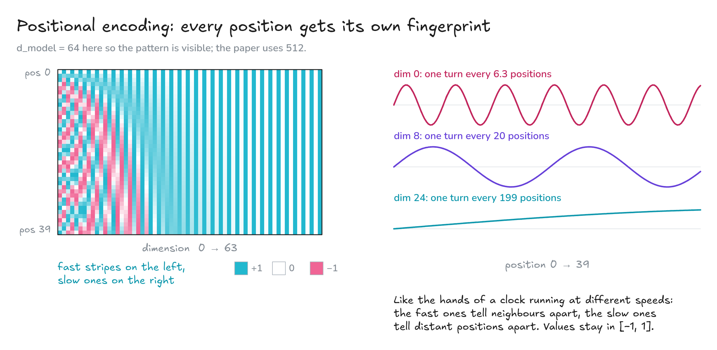
Fig. 9. The sinusoidal positional encoding as a heatmap (left) and three of its dimensions as waves (right)

Fig. 9. The sinusoidal positional encoding as a heatmap (left) and three of its dimensions as waves (right)

Two implementation notes. The table is stored with register_buffer, not nn.Parameter: it is saved with the model and moves to the GPU with it, but the optimizer never changes it. And the embeddings are multiplied by \(\sqrt{d_{model}}\) before the positions are added (Section 10.6), so that the position signal, which lives in \([-1, 1]\), does not drown out the token signal.

pos 1, dims 0-3: [0.8415, 0.5403, 0.8219, 0.5697]
cos(PE0, PE1) = 0.9731   cos(PE0, PE10) = 0.6789
dim   0: period = 6.3 positions
dim 128: period = 62.8 positions
dim 256: period = 628.3 positions
dim 510: period = 60,611.5 positions

Nearby positions have similar encodings (cosine similarity 0.97), and the similarity falls as the distance grows.

10.3 Multi-head attention

First the core formula from Section 4, written for tensors with any number of leading dimensions. A mask entry of 0 means “may not look here”:

# 2. Scaled dot-product attention -------------------------------------------------------
def scaled_dot_product_attention(Q, K, V, mask=None, dropout=None):
    """softmax(Q K^T / sqrt(d_k)) V. mask: 1 = may attend, 0 = blocked."""
    scores = Q @ K.transpose(-2, -1) / math.sqrt(Q.size(-1))
    if mask is not None:
        scores = scores.masked_fill(mask == 0, -1e9)   # -1e9, not -inf: a fully masked row stays finite
    weights = F.softmax(scores, dim=-1)
    if dropout is not None:
        weights = dropout(weights)                     # randomly drop some attention links in training
    return weights @ V, weights

Multi-head attention runs that formula in several smaller subspaces at once. The trick is a reshape, not a loop: with \(d_{model}=512\) and 8 heads, each head works in \(d_k=512/8=64\) dimensions, so the total cost matches a single 512-dimensional head.

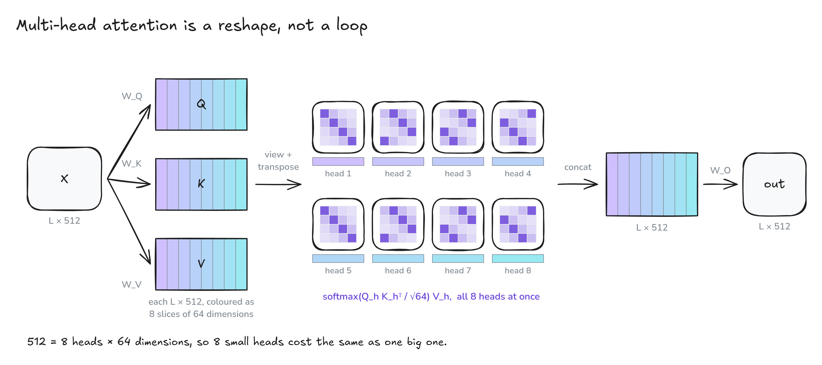
Fig. 10. One projection per role, split into 8 slices of 64; every head attends on its own slice, then the slices are put back together

Fig. 10. One projection per role, split into 8 slices of 64; every head attends on its own slice, then the slices are put back together

input             (B, L, 512)
W_Q, W_K, W_V     (B, L, 512)        three linear projections
view + transpose  (B, 8, L, 64)      8 heads, side by side
attention         (B, 8, L, 64)      all heads in parallel
transpose + view  (B, L, 512)        concatenate the heads
W_O               (B, L, 512)        mix them back together

# 3. Multi-head attention ---------------------------------------------------------------
class MultiHeadAttention(nn.Module):
    """Project, split into heads, attend in parallel, concatenate, project back."""
    def __init__(self, d_model, num_heads, dropout=0.1):
        super().__init__()
        assert d_model % num_heads == 0, "d_model must be divisible by num_heads"
        self.h, self.d_k = num_heads, d_model // num_heads
        self.W_Q = nn.Linear(d_model, d_model)
        self.W_K = nn.Linear(d_model, d_model)
        self.W_V = nn.Linear(d_model, d_model)
        self.W_O = nn.Linear(d_model, d_model)
        self.dropout = nn.Dropout(dropout)
        self.attn = None                                                   # last weights, for inspection

    def forward(self, query, key, value, mask=None):
        B = query.size(0)
        split = lambda x: x.view(B, -1, self.h, self.d_k).transpose(1, 2)  # (B, h, seq, d_k)
        Q, K, V = split(self.W_Q(query)), split(self.W_K(key)), split(self.W_V(value))
        if mask is not None:
            mask = mask.unsqueeze(1)                                       # same mask for every head
        out, self.attn = scaled_dot_product_attention(Q, K, V, mask, self.dropout)
        out = out.transpose(1, 2).contiguous().view(B, -1, self.h * self.d_k)  # concat heads
        return self.W_O(out)

10.4 Feed-forward network and Add & Norm

The feed-forward network widens each position to \(d_{ff}=2048\), applies a ReLU and narrows it back. Positions do not exchange information here; that is attention’s job. In Section 6’s words, attention lets residues talk and the feed-forward network lets each one think.

# 4. Position-wise feed-forward network -------------------------------------------------
class PositionwiseFeedForward(nn.Module):
    """Linear(d_model -> d_ff) -> ReLU -> Dropout -> Linear(d_ff -> d_model), per position."""
    def __init__(self, d_model, d_ff, dropout=0.1):
        super().__init__()
        self.linear1, self.linear2 = nn.Linear(d_model, d_ff), nn.Linear(d_ff, d_model)
        self.dropout = nn.Dropout(dropout)

    def forward(self, x):
        return self.linear2(self.dropout(F.relu(self.linear1(x))))

Every sub-layer, attention or feed-forward, is wrapped the same way: a residual shortcut adds the input back, and LayerNorm rescales each position’s vector to mean 0 and variance 1 (then applies a learned scale \(\gamma\) and shift \(\beta\)). The shortcut gives gradients a direct path through deep stacks; the normalization keeps the numbers in a stable range. LayerNorm, unlike BatchNorm, normalizes each position on its own, so it does not care about batch size or sequence length.

\[\text{Post-LN (paper):}\ \ \mathbf{x}\leftarrow\mathrm{LN}\big(\mathbf{x}+\mathrm{Sublayer}(\mathbf{x})\big)\qquad\text{Pre-LN (ESM-2, GPT-2):}\ \ \mathbf{x}\leftarrow\mathbf{x}+\mathrm{Sublayer}\big(\mathrm{LN}(\mathbf{x})\big)\]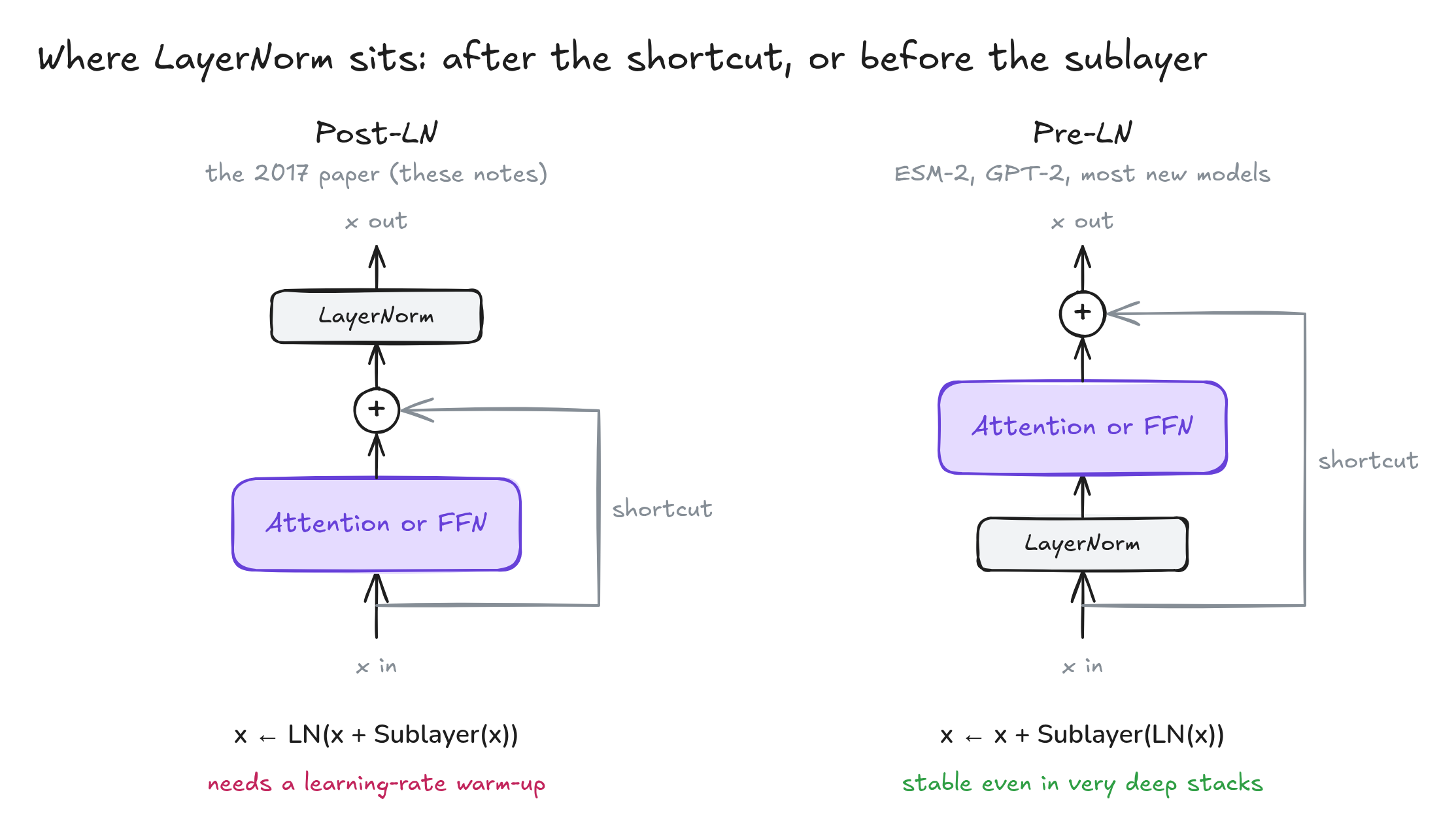

Fig. 11. Post-LN, as in the paper and these notes, and Pre-LN, as in ESM-2 (Section 6)

Fig. 11. Post-LN, as in the paper and these notes, and Pre-LN, as in ESM-2 (Section 6)

Pre-LN trains more stably in very deep stacks and needs little or no warm-up, which is why most modern models use it.

# 5. Add & Norm -------------------------------------------------------------------------
class LayerNorm(nn.Module):
    """gamma * (x - mean) / sqrt(var + eps) + beta, over the feature dimension."""
    def __init__(self, features, eps=1e-5):
        super().__init__()
        self.gamma = nn.Parameter(torch.ones(features))
        self.beta = nn.Parameter(torch.zeros(features))
        self.eps = eps

    def forward(self, x):
        mean = x.mean(-1, keepdim=True)
        var = x.var(-1, keepdim=True, unbiased=False)
        return self.gamma * (x - mean) / torch.sqrt(var + self.eps) + self.beta


class SublayerConnection(nn.Module):
    """Post-LN, as in the original paper: LayerNorm(x + Dropout(sublayer(x)))."""
    def __init__(self, d_model, dropout=0.1):
        super().__init__()
        self.norm, self.dropout = LayerNorm(d_model), nn.Dropout(dropout)

    def forward(self, x, sublayer):
        return self.norm(x + self.dropout(sublayer(x)))

10.5 Encoder and decoder layers

An encoder layer has two sub-layers; a decoder layer has three. The new one in the middle is cross-attention: its queries come from the decoder, its keys and values from the encoder’s output (the “memory”). That is how the sequence being written consults the sequence being read.

# 6. Encoder and decoder layers --------------------------------------------------------
class EncoderLayer(nn.Module):
    """Self-attention -> Add & Norm -> FFN -> Add & Norm."""
    def __init__(self, d_model, num_heads, d_ff, dropout=0.1):
        super().__init__()
        self.self_attn = MultiHeadAttention(d_model, num_heads, dropout)
        self.ffn = PositionwiseFeedForward(d_model, d_ff, dropout)
        self.sub1, self.sub2 = SublayerConnection(d_model, dropout), SublayerConnection(d_model, dropout)

    def forward(self, x, src_mask=None):
        x = self.sub1(x, lambda x: self.self_attn(x, x, x, src_mask))     # Q = K = V = x
        return self.sub2(x, self.ffn)


class DecoderLayer(nn.Module):
    """Masked self-attention -> Add & Norm -> cross-attention -> Add & Norm -> FFN -> Add & Norm."""
    def __init__(self, d_model, num_heads, d_ff, dropout=0.1):
        super().__init__()
        self.self_attn = MultiHeadAttention(d_model, num_heads, dropout)
        self.cross_attn = MultiHeadAttention(d_model, num_heads, dropout)
        self.ffn = PositionwiseFeedForward(d_model, d_ff, dropout)
        self.sub1, self.sub2, self.sub3 = (SublayerConnection(d_model, dropout) for _ in range(3))

    def forward(self, x, memory, src_mask=None, tgt_mask=None):
        x = self.sub1(x, lambda x: self.self_attn(x, x, x, tgt_mask))     # look back only
        x = self.sub2(x, lambda x: self.cross_attn(x, memory, memory, src_mask))  # Q: decoder, K/V: encoder
        return self.sub3(x, self.ffn)

	Encoder layer	Decoder layer
Self-attention	Sees every position (only padding is masked)	Sees only earlier positions (causal mask)
Cross-attention	None	Queries from the decoder, keys and values from the encoder
Feed-forward	Yes	Yes
Add & Norm blocks	2	3

10.6 The stacks

Each stack is an embedding (scaled by \(\sqrt{d_{model}}\)), the positional encoding, and \(N\) identical layers. Stacking lets each layer build on what the previous one gathered.

# 7. Stacks -----------------------------------------------------------------------------
class Encoder(nn.Module):
    def __init__(self, vocab_size, d_model, num_heads, d_ff, num_layers, dropout=0.1, max_len=5000):
        super().__init__()
        self.d_model = d_model
        self.embed = nn.Embedding(vocab_size, d_model)
        self.pos = PositionalEncoding(d_model, dropout, max_len)
        self.layers = nn.ModuleList(EncoderLayer(d_model, num_heads, d_ff, dropout) for _ in range(num_layers))

    def forward(self, src, src_mask=None):
        x = self.pos(self.embed(src) * math.sqrt(self.d_model))            # scale, then add positions
        for layer in self.layers:
            x = layer(x, src_mask)
        return x


class Decoder(nn.Module):
    def __init__(self, vocab_size, d_model, num_heads, d_ff, num_layers, dropout=0.1, max_len=5000):
        super().__init__()
        self.d_model = d_model
        self.embed = nn.Embedding(vocab_size, d_model)
        self.pos = PositionalEncoding(d_model, dropout, max_len)
        self.layers = nn.ModuleList(DecoderLayer(d_model, num_heads, d_ff, dropout) for _ in range(num_layers))

    def forward(self, tgt, memory, src_mask=None, tgt_mask=None):
        x = self.pos(self.embed(tgt) * math.sqrt(self.d_model))
        for layer in self.layers:
            x = layer(x, memory, src_mask, tgt_mask)
        return x

10.7 Masks, “shifted right”, and the full model

The decoder is trained with teacher forcing: it is shown the correct output so far and asked for the next token. Its input is the target shifted one step to the right, behind a start token. If the decoder were writing a CDR3:

Decoder input	`<bos>`	C	A	S	S	…
Target	C	A	S	S	I	…

On its own, the shift is not enough, because self-attention could still peek at later inputs. The causal mask forbids that: row \(i\) of the lower-triangular matrix lets position \(i\) see positions \(0\ldots i\) only, exactly the \(M\) of Section 7. A padding mask hides the filler tokens that make sequences of different lengths fit in one batch. At inference time there is no target, so the decoder starts from <bos>, picks the most likely token, appends it and repeats until it writes <eos> (greedy decoding; beam search keeps several candidates instead of one).

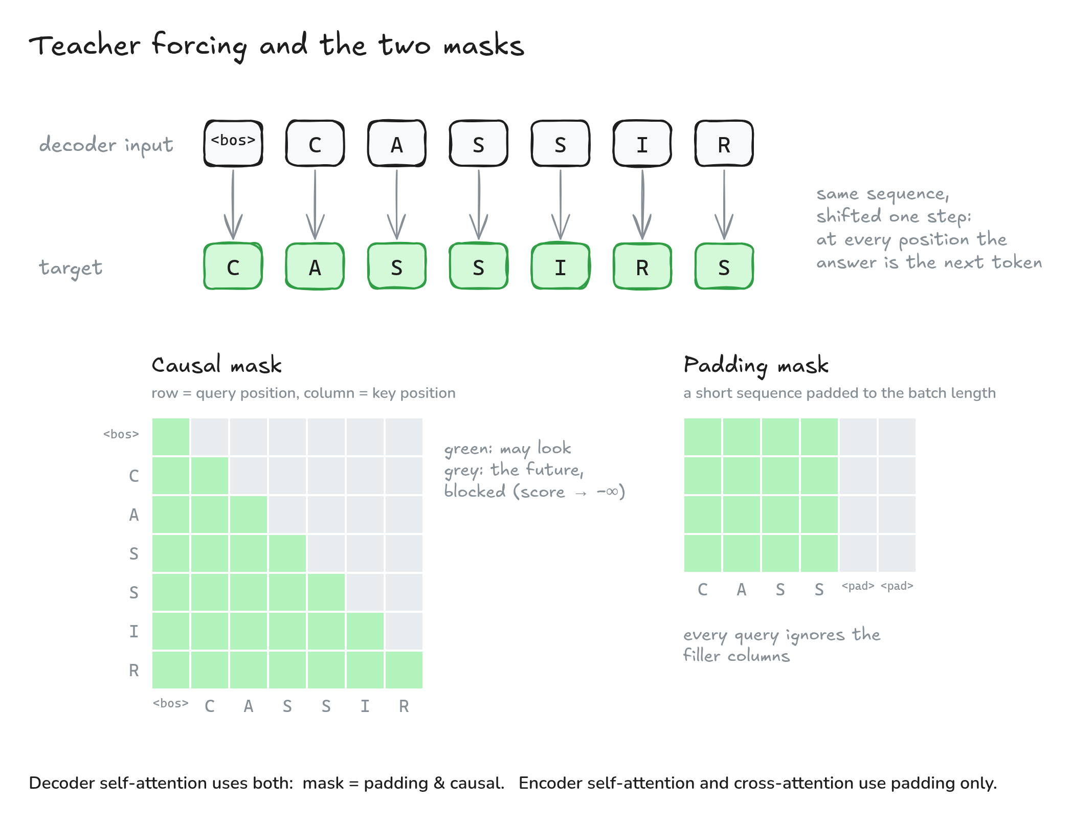
Fig. 12. Top: teacher forcing, where the decoder input is the target shifted one step right. Bottom: the causal and padding masks (green = may attend)

Fig. 12. Top: teacher forcing, where the decoder input is the target shifted one step right. Bottom: the causal and padding masks (green = may attend)

# 8. The full model, masks and greedy decoding -----------------------------------------
class Transformer(nn.Module):
    def __init__(self, src_vocab, tgt_vocab, d_model=512, num_heads=8, d_ff=2048,
                 num_layers=6, dropout=0.1, max_len=5000):
        super().__init__()
        self.encoder = Encoder(src_vocab, d_model, num_heads, d_ff, num_layers, dropout, max_len)
        self.decoder = Decoder(tgt_vocab, d_model, num_heads, d_ff, num_layers, dropout, max_len)
        self.generator = nn.Linear(d_model, tgt_vocab)                     # logits over the vocabulary
        for p in self.parameters():
            if p.dim() > 1:
                nn.init.xavier_uniform_(p)

    def encode(self, src, src_mask=None):
        return self.encoder(src, src_mask)

    def decode(self, tgt, memory, src_mask=None, tgt_mask=None):
        return self.generator(self.decoder(tgt, memory, src_mask, tgt_mask))

    def forward(self, src, tgt, src_mask=None, tgt_mask=None):
        return self.decode(tgt, self.encode(src, src_mask), src_mask, tgt_mask)


def padding_mask(seq, pad_idx=0):                   # (B, 1, len): hide padding keys
    return (seq != pad_idx).unsqueeze(1)

def causal_mask(size, device=None):                 # (1, size, size): lower triangle
    return torch.tril(torch.ones(size, size, dtype=torch.bool, device=device)).unsqueeze(0)

def make_masks(src, tgt_in, pad_idx=0):
    return padding_mask(src, pad_idx), padding_mask(tgt_in, pad_idx) & causal_mask(tgt_in.size(1), tgt_in.device)

@torch.no_grad()
def greedy_decode(model, src, max_len, bos, eos, pad_idx=0):
    model.eval()
    src_mask = padding_mask(src, pad_idx)
    memory = model.encode(src, src_mask)
    ys = torch.full((src.size(0), 1), bos, dtype=torch.long, device=src.device)
    for _ in range(max_len):
        logits = model.decode(ys, memory, src_mask, causal_mask(ys.size(1), src.device))
        next_tok = logits[:, -1].argmax(-1, keepdim=True)                 # most likely next token
        ys = torch.cat([ys, next_tok], dim=1)
        if (next_tok == eos).all():
            break
    return ys

10.8 Check it, and count the parameters

Before trusting hand-written modules, compare them with PyTorch’s own. With the same weights copied in, my LayerNorm matches nn.LayerNorm and my MultiHeadAttention matches nn.MultiheadAttention, causal mask included. Then build the base model from the paper (here with a 10,000-token source vocabulary and an 8,000-token target vocabulary) and push a batch through it:

max |LayerNorm - nn.LayerNorm| = 2.4e-07
max |ours - nn.MultiheadAttention| (causal) = 0.0e+00
parameters: total 57,458,496 | one encoder layer 3,152,384 | one decoder layer 4,204,032
src_mask (2, 1, 10) tgt_mask (2, 12, 12) logits (2, 12, 8000)

Where the 57 million weights sit:

Part	Weights	Count
Attention, per sub-layer	\(4d^2+4d\)	1,050,624
Feed-forward, per layer	\(2\,d\,d_{ff}+d_{ff}+d\)	2,099,712
Encoder layer	1 attention + 1 FFN + 2 LayerNorms	3,152,384
Decoder layer	2 attentions + 1 FFN + 3 LayerNorms	4,204,032
6 + 6 layers		44,138,496
Embeddings and output projection	\((10{,}000+8{,}000)\,d\) + \(8{,}000\,(d+1)\)	13,320,000

Inside each encoder layer, two thirds of the weights are in the feed-forward network, as the last row of the myth table in Section 9 says.

10.9 Train it: teach a Transformer to read a CDR3 backwards

A copy task is the “hello world” of sequence-to-sequence models: the right answer is known, so you can see at once whether every piece is wired correctly. Here a small model (2 layers, \(d_{model}=64\), 4 heads) learns to reverse random amino-acid strings of 8–16 residues. Training uses the paper’s recipe: Adam with \(\beta_2=0.98\), a learning rate that warms up and then decays,

\[\mathrm{lr}=d_{model}^{-0.5}\cdot\min\!\left(\mathrm{step}^{-0.5},\ \mathrm{step}\cdot\mathrm{warmup}^{-1.5}\right),\]

label smoothing of 0.1 (the target puts 90% on the right token and spreads the rest), dropout of 0.1 and gradient clipping.

import time
torch.manual_seed(0)

AA = "ACDEFGHIKLMNPQRSTVWY"
PAD, BOS, EOS = 0, 1, 2
stoi = {a: i + 3 for i, a in enumerate(AA)}
itos = {i: a for a, i in stoi.items()}
V = len(AA) + 3

def batch(n, lo=8, hi=16):
    """Random amino-acid strings; the target is the same string reversed."""
    lens = torch.randint(lo, hi + 1, (n,))
    src = torch.full((n, hi), PAD); tgt = torch.full((n, hi + 2), PAD)
    for b, L in enumerate(lens):
        s = torch.randint(3, V, (L,))
        src[b, :L] = s
        tgt[b, 0], tgt[b, 1:L + 1], tgt[b, L + 1] = BOS, s.flip(0), EOS
    return src, tgt

model = Transformer(V, V, d_model=64, num_heads=4, d_ff=256, num_layers=2, dropout=0.1)
opt = torch.optim.Adam(model.parameters(), lr=1.0, betas=(0.9, 0.98), eps=1e-9)
warmup = 400
sched = torch.optim.lr_scheduler.LambdaLR(           # the paper's schedule: warm up, then 1/sqrt(step)
    opt, lambda s: 64 ** -0.5 * min((s + 1) ** -0.5, (s + 1) * warmup ** -1.5))
loss_fn = nn.CrossEntropyLoss(ignore_index=PAD, label_smoothing=0.1)

t0 = time.time()
for step in range(1, 3001):
    model.train()
    src, tgt = batch(128)
    tgt_in, tgt_out = tgt[:, :-1], tgt[:, 1:]        # "shifted right": predict token t+1 from tokens <= t
    src_mask, tgt_mask = make_masks(src, tgt_in)
    logits = model(src, tgt_in, src_mask, tgt_mask)
    loss = loss_fn(logits.reshape(-1, V), tgt_out.reshape(-1))
    opt.zero_grad(); loss.backward()
    nn.utils.clip_grad_norm_(model.parameters(), 1.0)
    opt.step(); sched.step()
    if step % 500 == 0:
        print(f"step {step:4d}  loss {loss.item():.3f}")
print(f"training time: {time.time() - t0:.0f} s")

src, tgt = batch(1000)
out = greedy_decode(model, src, max_len=18, bos=BOS, eos=EOS)
ok = sum(out[b, 1:len(tgt[b].nonzero())].tolist() == tgt[b, 1:len(tgt[b].nonzero())].tolist() for b in range(1000))
print(f"held-out sequences reversed exactly: {ok}/1000")

cdr3 = "CASSIRSSYEQYF"
src = torch.tensor([[stoi[a] for a in cdr3]])
out = greedy_decode(model, src, max_len=18, bos=BOS, eos=EOS)[0, 1:].tolist()
print("input :", cdr3)
print("output:", "".join(itos[i] for i in out if i not in (EOS, PAD)))

step  500  loss 0.905
step 1000  loss 0.697
step 1500  loss 0.670
step 2000  loss 0.660
step 2500  loss 0.639
step 3000  loss 0.627
training time: 250 s
held-out sequences reversed exactly: 999/1000
input : CASSIRSSYEQYF
output: FYQEYSSRISSAC

After about four minutes on a CPU, the model reverses 999 of 1,000 sequences it has never seen, including our CDR3β. The loss levels off near 0.6 rather than 0 because of label smoothing: even a perfect prediction is scored against a target that is only 90% sure.

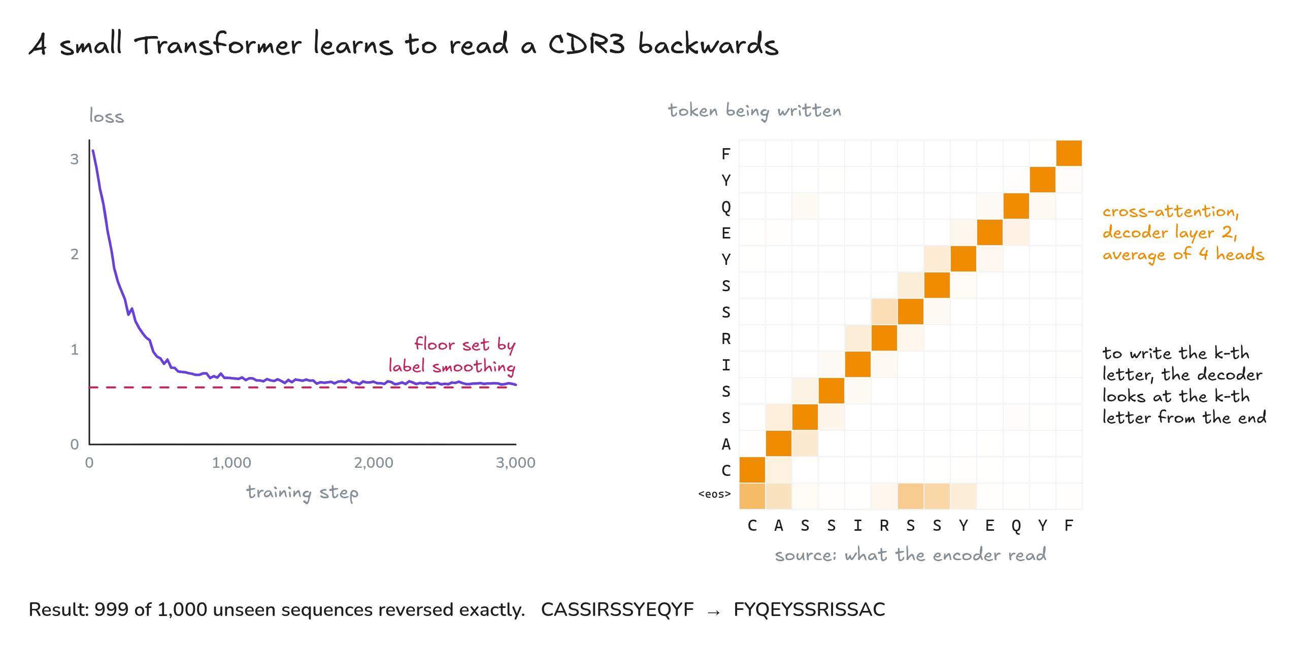
Fig. 13. Left: the training loss. Right: the trained model's cross-attention while it writes the reversed CDR3β

Fig. 13. Left: the training loss. Right: the trained model’s cross-attention while it writes the reversed CDR3β

Fig. 13 opens the trained model up. In the second decoder layer, cross-attention lines up along an anti-diagonal: to write the k-th letter of the answer, the decoder puts on average 95% of its attention on the k-th letter from the end of the source. Nobody wrote that rule into the model; it found it from examples. This is the same mechanism a translation model uses to align words, and a TCR–peptide model to align residues.

The training tricks from the paper, in one place:

Trick	What it does
Learning-rate warm-up	Small steps while the weights are still random, then a \(1/\sqrt{\mathrm{step}}\) decay. Post-LN models often diverge without it.
Label smoothing	Softens the one-hot target, which discourages over-confidence and improves generalization.
Dropout (0.1)	On the attention weights, the feed-forward activations, each sub-layer’s output before the residual add, and the embeddings plus positions.
Gradient clipping	Caps the gradient norm so one bad batch cannot blow up the weights.
Xavier initialization	Starts each weight matrix at a scale that keeps signals from shrinking or exploding.
Beam search	At inference, keeps the k best partial outputs instead of only the single best.

The toy weights are set by hand so that each head is easy to read; trained models learn theirs from data. The cross-attention map in Fig. 6 is illustrative. ESM-2 probabilities are renormalized over the 20 standard amino acids. Figures were drawn with Excalidraw; the editable sources open directly on excalidraw.com: Fig. 1, Fig. 2, Fig. 3, Fig. 4, Fig. 5, Fig. 6, Fig. 7, Fig. 8, Fig. 9, Fig. 10, Fig. 11, Fig. 12, Fig. 13. Fig. 13 uses the real attention weights of the model trained in Section 10.9. The video was animated with Remotion and narrated with a synthetic (text-to-speech) voice. Music: “Deliberate Thought” by Kevin MacLeod (incompetech.com), licensed under CC BY 4.0.