In one sentence: a survival curve shows the share of patients still event-free over time, estimated step by step, using every patient for exactly as long as they were followed.
\[\hat S(t)=\prod_{t_i\le t}\left(1-\frac{d_i}{n_i}\right)\]A tick mark is not a death, and a hazard ratio of 0.70 does not mean “30% longer life”.
The running example is a simulated phase 3 trial. 400 patients with advanced cancer are randomized to a new immunotherapy or to chemotherapy and followed for overall survival. The data are made up for teaching. The Python script at the end reproduces every number in this article and in the companion video.
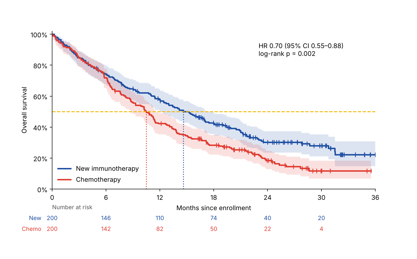
Fig. 1. The picture behind a headline like “new drug cuts the risk of death by 30%”: steps, tick marks, shaded bands, a table of numbers under the axis, and an HR. By the end of this article you can read all of them.
1. Time to an event
A survival curve answers one question: how long until something happens? The event depends on the study. It can be death from any cause (overall survival, OS), tumor growth or death (progression-free survival, PFS), relapse, or even a good event such as recovery. Time zero is usually randomization or enrollment.
Every patient carries a clock (Fig. 2). Patients join on different dates, but the analysis happens at one data cut-off, so we reset every clock to start at zero. Some clocks end with the event (●). Others just stop: the patient moved away, was lost to follow-up, or was still alive at the cut-off. That is censoring (+). We know the patient survived at least that long (\(T > c\)), and nothing more.
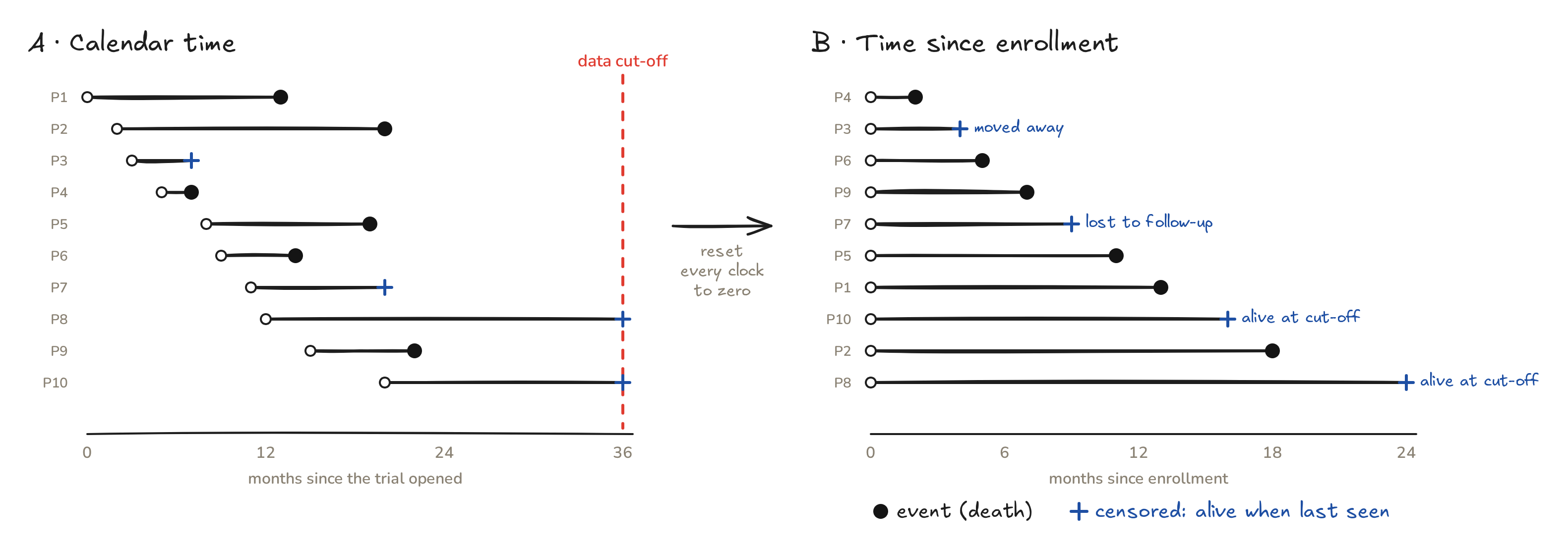
Fig. 2. Ten patients from the new-drug arm. Left: calendar time with one data cut-off. Right: the same follow-up, measured from each patient’s own enrollment.
2. Why not just count?
What fraction of these ten patients survived one year? At 12 months, 4 had died, 2 had been censored (at months 4 and 9), and 4 were still being followed.
| Shortcut | 1-year survival | What goes wrong |
|---|---|---|
| Drop the 2 censored patients | 4/8 = 50% | throws away months of real follow-up |
| Count them as deaths | 4/10 = 40% | “kills” two people last seen alive |
| Kaplan–Meier | 54% | uses every patient for as long as we watched them |
Both shortcuts push the answer down. In a real trial, with hundreds of patients and heavy censoring, the error can be large.
3. Kaplan–Meier, step by step
In 1958, Edward Kaplan and Paul Meier showed how to use censored follow-up correctly. Think of survival as a column shared equally by everyone still being followed (Fig. 3):
- Start: 10 patients, so 10 shares of 10% each.
- Month 2: a patient dies. Their share falls away, and the curve steps down to 90%.
- Month 4: a patient is censored. Nobody died, so the curve stays flat. But now 8 people share the 90%, so each share grows to 11.25%.
- Month 5: the next death removes a bigger share: 90% × (1 − 1/8) = 78.75%.
Each drop multiplies the current survival by \(1-d_i/n_i\), where \(d_i\) is the number of deaths at that time and \(n_i\) the number of patients still at risk just before it. Censored patients never cause a drop; they only leave the risk set. Statisticians call this view redistribution to the right (Efron, 1967): a censored patient’s share passes to the patients who are still being followed.
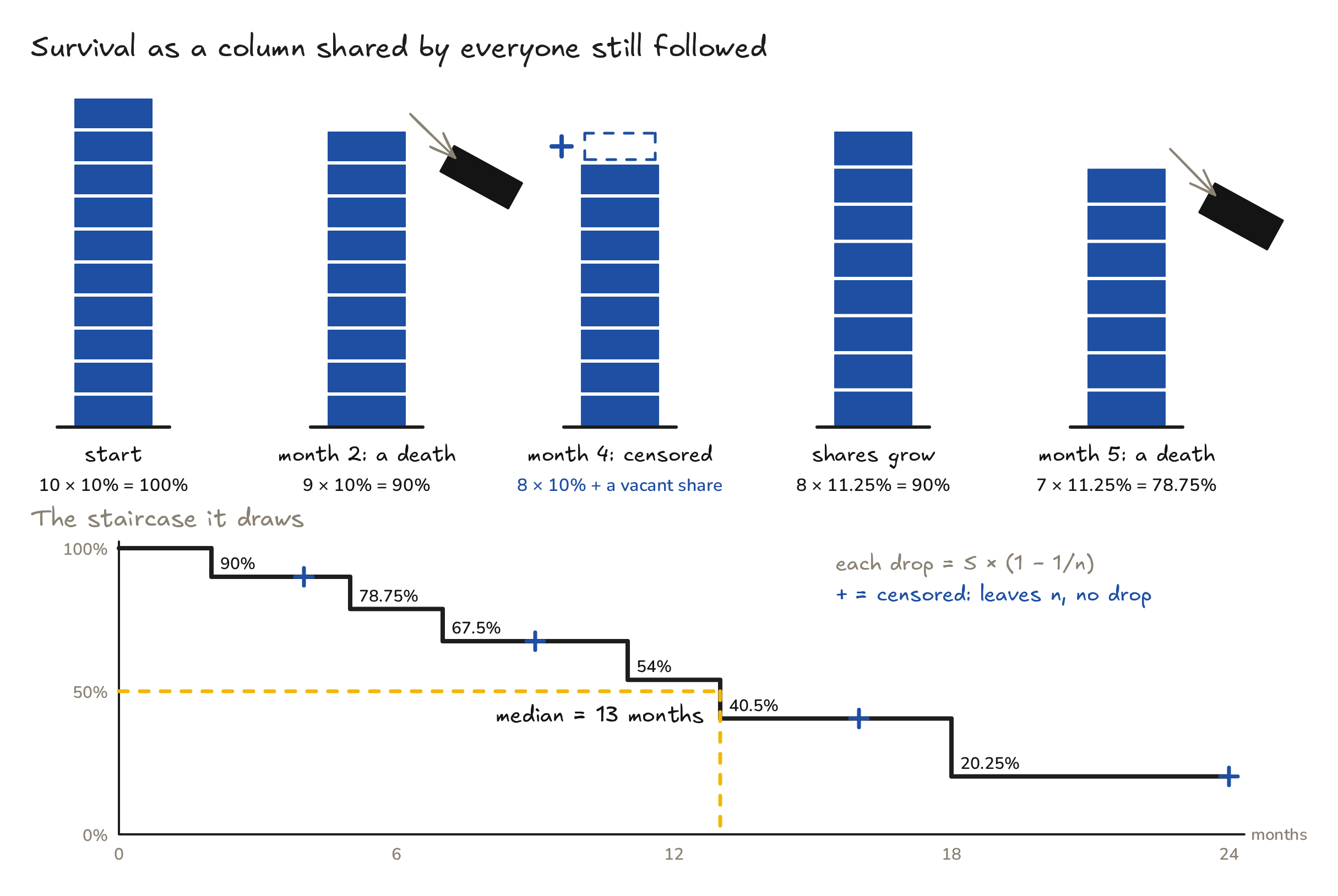
Fig. 3. Every patient at risk holds an equal share of the survival column. A death removes a share; a censoring makes the remaining shares bigger. The top of the column traces the Kaplan–Meier staircase.
The full hand calculation:
| \(t_i\) (months) | \(n_i\) at risk | \(d_i\) deaths | \(1-d_i/n_i\) | \(\hat S(t_i)\) |
|---|---|---|---|---|
| 2 | 10 | 1 | 9/10 | 0.9000 |
| 5 | 8 | 1 | 7/8 | 0.7875 |
| 7 | 7 | 1 | 6/7 | 0.6750 |
| 11 | 5 | 1 | 4/5 | 0.5400 |
| 13 | 4 | 1 | 3/4 | 0.4050 |
| 18 | 2 | 1 | 1/2 | 0.2025 |
Notice that \(n_i\) jumps from 10 to 8 between months 2 and 5: one death, plus one censoring. At one year, \(\hat S(12) = 0.54\).
4. The formula, the median and the uncertainty
Formally, the survival function is the probability of surviving beyond time \(t\),
\[S(t) = P(T > t),\]and the Kaplan–Meier estimator multiplies over all event times up to \(t\):
\[\hat S(t) = \prod_{t_i \le t}\left(1 - \frac{d_i}{n_i}\right).\]- Median survival is the first time the curve reaches 50% or below: 13 months for these ten patients. If the curve never gets down to 50%, papers report the median as “not reached” (NR).
- Landmark survival is the height of the curve at a fixed time, for example 1-year or 2-year survival.
- Uncertainty. Greenwood’s formula estimates the variance: \(\widehat{\mathrm{Var}}\big[\hat S(t)\big] = \hat S(t)^2 \sum_{t_i \le t}\frac{d_i}{n_i(n_i-d_i)}.\) The 95% band is usually built on a transformed scale, log or \(\log(-\log)\), so that it stays between 0 and 1. The script below uses \(\log(-\log)\), as lifelines does. The fewer patients at risk, the wider the band.
- The key assumption is non-informative censoring: patients who leave the study must have the same outlook as those who stay. If the sickest patients drop out, the curve looks better than the truth.
5. Comparing two arms
Now the whole simulated trial (Figs. 1 and 4). There are 200 patients per arm, with 135 deaths on the new drug and 160 on chemotherapy.
- Read vertically to compare survival at a fixed time. At 2 years: 30.3% (95% CI 23.6–37.3%) vs 18.4% (12.9–24.7%).
- Read horizontally to compare medians: 14.6 months (95% CI 12.0–17.5) vs 10.5 months (8.7–11.5), a gain of 4.1 months.
- Read the numbers at risk. At 30 months only 20 and 4 patients remain. The right-hand tail is thin, and its bands are wide.
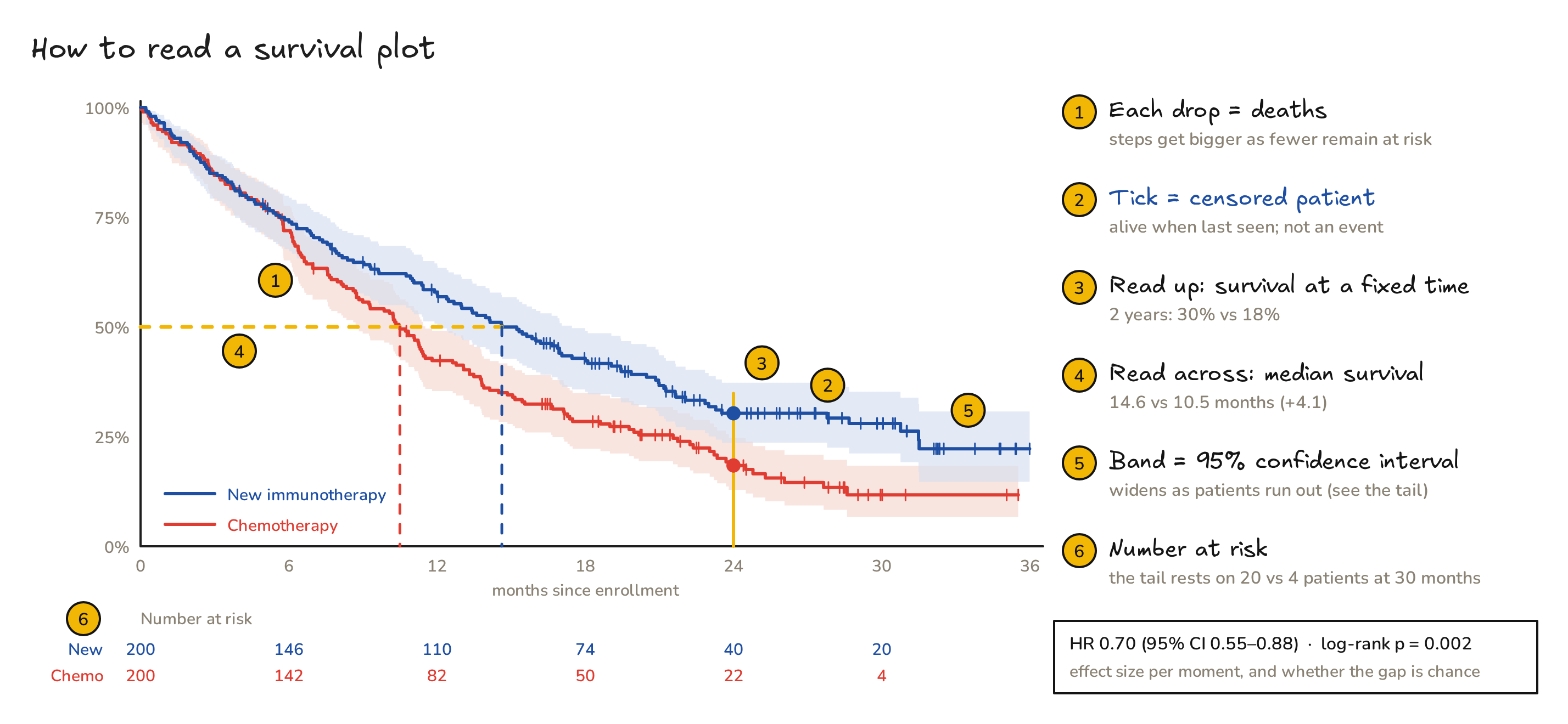
Fig. 4. A six-point checklist for any published Kaplan–Meier plot.
6. Is the gap real? The log-rank test and the hazard ratio
The log-rank test walks through every death. At each one it asks: if the drug did nothing, how many of these deaths should have happened in the new-drug arm, given how many patients each arm still had at risk? It then compares that expected count with the observed count.
\[E_1 = \sum_i d_i\,\frac{n_{1i}}{n_i},\qquad V_1=\sum_i d_i\,\frac{n_{1i}}{n_i}\Big(1-\frac{n_{1i}}{n_i}\Big)\frac{n_i-d_i}{n_i-1},\qquad \chi^2 = \frac{(O_1-E_1)^2}{V_1}\]The new-drug arm was expected to have \(E_1 = 161.2\) deaths and had \(O_1 = 135\). That gives \(\chi^2 = 9.51\) with 1 degree of freedom, so p = 0.002. The test says that the curves differ. It does not say by how much.
The hazard is the instantaneous event rate among those still at risk:
\[h(t) = \lim_{\Delta t\to 0}\frac{P(t \le T < t+\Delta t \mid T \ge t)}{\Delta t},\qquad S(t) = \exp\Big(-\int_0^t h(u)\,du\Big).\]The hazard ratio comes from the Cox proportional hazards model, \(h(t\mid x) = h_0(t)\,e^{\beta x}\), with \(x = 1\) for the new drug:
\[\mathrm{HR} = \frac{h_{\text{new}}(t)}{h_{\text{chemo}}(t)} = e^{\beta} = 0.70\quad(95\%\ \text{CI } 0.55\text{–}0.88).\]At any moment, a patient on the new drug dies at about 70% of the chemotherapy rate. That is the “30% lower risk of death” in the headline. If the ratio really is constant over time, the two curves are tied together exactly:
\[S_{\text{new}}(t) = S_{\text{chemo}}(t)^{\mathrm{HR}}\quad\Rightarrow\quad 0.18^{0.70} = 0.30,\]which matches the observed 2-year survival of 0.30. With unrounded inputs, \(0.184^{0.697} = 0.31\), still close.
7. Traps
| Myth | Truth |
|---|---|
| A tick mark is a death. | A tick is a censored patient, alive when last seen. Only drops are events. |
| HR 0.70 means living 30% longer. | The HR compares the risk at each moment. Here the median gain is 4.1 months (+39%), and mean survival within 2 years (the RMST) gains 2.2 months: 14.3 vs 12.1. |
| A flat tail means a cure, or certainty. | The tail rests on few patients (20 vs 4 at 30 months). Check the numbers at risk and the width of the band. |
| One HR summarizes any two curves. | If the curves cross or separate late (common with immunotherapy), the hazards are not proportional. Compare survival at fixed times, or the area under the curves (RMST). |
| “Median not reached” means everyone survives. | It only means that fewer than half the patients have had the event so far. |
| Curves from different trials can be compared. | Patients, endpoints and time zero differ between trials. Compare arms within one randomized trial. |
8. Cheat sheet
| Term | Meaning |
|---|---|
| Event / endpoint | what the clock waits for (OS: death from any cause; PFS: progression or death) |
| Time zero | when the clock starts (randomization, enrollment, diagnosis) |
| Censored (+) | follow-up stopped without the event; we know only that \(T > c\) |
| At risk, \(n_i\) | patients still followed and event-free just before \(t_i\) |
| \(S(t)\) | probability of being event-free beyond time \(t\) |
| Kaplan–Meier | \(\hat S(t)=\prod(1-d_i/n_i)\), a step function that drops only at events |
| Median survival | first \(t\) with \(\hat S(t)\le 0.5\) |
| Landmark survival | \(\hat S\) at a fixed time, such as 2-year OS |
| 95% band | uncertainty from Greenwood’s variance; widens as \(n\) shrinks |
| Log-rank test | observed vs expected events: is there a difference? |
| Hazard, \(h(t)\) | instantaneous event rate among those still at risk |
| Hazard ratio | \(h_1(t)/h_0(t)\) from a Cox model; below 1 favors arm 1 |
| RMST | area under \(\hat S(t)\) up to a time \(\tau\): mean event-free time within \(\tau\) |
9. Try it yourself: survival analysis from scratch
The script uses only NumPy, plus Matplotlib for the plot. It redoes the hand table, simulates the trial with the same random seed as the video, and computes the Kaplan–Meier curves, Greenwood bands, medians, the log-rank test and the Cox hazard ratio. It also draws Fig. 1.
"""Survival curves from scratch: Kaplan–Meier, log-rank test and Cox hazard ratio with NumPy only.
Simulated teaching data: a two-arm trial, new immunotherapy (arm 1) vs chemotherapy (arm 0), 200 patients per arm."""
import numpy as np
from math import erf, exp, log, sqrt

def kaplan_meier(time, event):
    """Return event times t_i, numbers at risk n_i, deaths d_i and S(t_i) = prod(1 - d_i/n_i)."""
    time, event = np.asarray(time, float), np.asarray(event, int)
    t = np.unique(time[event == 1])                                   # distinct event times
    n = np.array([(time >= ti).sum() for ti in t])                    # at risk just before t_i
    d = np.array([((time == ti) & (event == 1)).sum() for ti in t])   # deaths at t_i
    return t, n, d, np.cumprod(1 - d / n)

def greenwood_ci(n, d, S, z=1.96):
    """95% CI with Greenwood's variance on the log(-log S) scale."""
    se = np.sqrt(np.cumsum(d / (n * (n - d)))) / np.abs(np.log(S))
    return S ** np.exp(z * se), S ** np.exp(-z * se)

def S_at(t, S, x):                       # read the step function at time x
    i = np.searchsorted(t, x, side='right') - 1
    return 1.0 if i < 0 else S[i]

def median(t, S):                        # first time the curve reaches 50% or below
    return t[np.argmax(S <= 0.5)] if (S <= 0.5).any() else None

def logrank(time, event, group):
    """Observed vs expected deaths in group 1 at every event time, then chi-square with 1 df."""
    O = E = V = 0.0
    for ti in np.unique(time[event == 1]):
        at = time >= ti; n = at.sum(); n1 = (at & (group == 1)).sum()
        dd = (time == ti) & (event == 1); d = dd.sum()
        O += (dd & (group == 1)).sum(); E += d * n1 / n
        V += d * (n1 / n) * (1 - n1 / n) * (n - d) / (n - 1) if n > 1 else 0.0
    chi2 = (O - E) ** 2 / V
    return O, E, chi2, 1 - erf(sqrt(chi2 / 2))      # p = upper tail of chi-square(1)

def cox_hr(time, event, x, iters=25):
    """Cox model with one 0/1 covariate, fitted by Newton-Raphson on the partial likelihood."""
    o = np.argsort(-time); e, x = event[o], x[o].astype(float)     # sort by time, latest first
    b = 0.0
    for _ in range(iters):
        w = np.exp(b * x); p = np.cumsum(w * x) / np.cumsum(w)       # share of 'new' in each risk set
        U, I = np.sum(e * (x - p)), np.sum(e * p * (1 - p))          # score and information
        b += U / I
    se = 1 / sqrt(I)
    return exp(b), exp(b - 1.96 * se), exp(b + 1.96 * se)

# ---- 1. ten patients by hand (new-drug arm): follow-up in months, 1 = died, 0 = censored --------------
mini_t = np.array([13, 18, 4, 2, 11, 5, 9, 24, 7, 16]); mini_e = np.array([1, 1, 0, 1, 1, 1, 0, 0, 1, 0])
t, n, d, S = kaplan_meier(mini_t, mini_e)
for row in zip(t, n, d, S): print('t=%2d  n=%2d  d=%d  S=%.4f' % row)
print('S(12) = %.2f   median = %d months' % (S_at(t, S, 12), median(t, S)))

# ---- 2. the full simulated trial ------------------------------------------------------------------------
rng = np.random.default_rng(5427)
lam0, hr_true, lam_drop = log(2) / 10.0, 0.70, -log(0.95) / 12      # chemo median 10 mo, 5% drop-out per year
arm, time, event = [], [], []
for a in (1, 0):
    m = 200 - (10 if a == 1 else 0)                                  # arm 1 already holds the ten patients above
    enrol = rng.uniform(0, 20, m)                                    # enrolment spread over 20 months
    T = rng.exponential(1 / (lam0 * (hr_true if a == 1 else 1.0)), m)  # true time to death
    D = rng.exponential(1 / lam_drop, m)                             # time to drop-out
    C = 36 - enrol                                                   # data cut-off at month 36
    tt, ee = np.minimum(np.minimum(T, D), C), (T <= np.minimum(D, C)).astype(int)
    if a == 1: tt, ee = np.r_[mini_t, tt], np.r_[mini_e, ee]
    arm += [a] * 200; time += list(tt); event += list(ee)
arm, time, event = np.array(arm), np.array(time), np.array(event)

fits = {}
for a, name in ((1, 'new'), (0, 'chemo')):
    t, n, d, S = kaplan_meier(time[arm == a], event[arm == a]); fits[name] = (t, n, d, S)
    lo, hi = greenwood_ci(n, d, S); i24 = np.searchsorted(t, 24, side='right') - 1
    risk = [int((time[arm == a] >= x).sum()) for x in (0, 6, 12, 18, 24, 30)]
    print('%-5s events %d  median %.1f  S(12) %.3f  S(24) %.3f (95%% CI %.3f-%.3f)  at risk %s'
          % (name, event[arm == a].sum(), median(t, S), S_at(t, S, 12), S[i24], lo[i24], hi[i24], risk))
O, E, chi2, p = logrank(time, event, arm)
hr, hr_lo, hr_hi = cox_hr(time, event, arm)
print('log-rank: observed %d vs expected %.1f deaths, chi2 = %.2f, p = %.4f' % (O, E, chi2, p))
print('hazard ratio %.2f (95%% CI %.2f-%.2f)' % (hr, hr_lo, hr_hi))
print('proportional hazards check: 0.18 ** 0.70 = %.2f' % (0.18 ** 0.70))

# ---- 3. the plot: steps, censor ticks, 95% bands, numbers at risk ----------------------------------------
import matplotlib; matplotlib.use('Agg'); import matplotlib.pyplot as plt
fig, ax = plt.subplots(figsize=(9, 5.6), dpi=160)
for a, name, col, lab in ((1, 'new', '#1E4FA3', 'New immunotherapy'), (0, 'chemo', '#E03C31', 'Chemotherapy')):
    t, n, d, S = fits[name]; lo, hi = greenwood_ci(n, d, S)
    x = np.r_[0, t, time[arm == a].max()]; y = np.r_[1, S, S[-1]]
    ax.step(x, y, where='post', color=col, lw=2.2, label=lab)
    ax.fill_between(x, np.r_[1, lo, lo[-1]], np.r_[1, hi, hi[-1]], step='post', color=col, alpha=0.15, lw=0)
    c = time[(arm == a) & (event == 0)]; ax.plot(c, [S_at(t, S, ci) for ci in c], '|', color=col, ms=7, mew=1.2)
    m = median(t, S); ax.plot([m, m], [0, 0.5], ':', color=col, lw=1.4)
    for k, xx in enumerate((0, 6, 12, 18, 24, 30)):
        ax.text(xx, -0.20 - 0.07 * (a == 0), str((time[arm == a] >= xx).sum()), color=col, ha='center', fontsize=9)
ax.axhline(0.5, color='#F2B705', lw=1.4, ls='--')
ax.text(-1.2, -0.20, 'New', ha='right', fontsize=9, color='#1E4FA3'); ax.text(-1.2, -0.27, 'Chemo', ha='right', fontsize=9, color='#E03C31')
ax.text(0, -0.13, 'Number at risk', fontsize=9, color='#555')
ax.text(23, 0.86, 'HR %.2f (95%% CI %.2f–%.2f)\nlog-rank p = %.3f' % (hr, hr_lo, hr_hi, p), fontsize=10)
ax.set(xlim=(0, 36), ylim=(0, 1.02), xticks=range(0, 37, 6), xlabel='Months since enrollment', ylabel='Overall survival')
ax.yaxis.set_major_formatter(matplotlib.ticker.PercentFormatter(1.0)); ax.legend(loc='lower left', frameon=False)
ax.spines[['top', 'right']].set_visible(False); fig.subplots_adjust(bottom=0.27)
fig.savefig('figures/fig1_trial_km.png'); print('saved figures/fig1_trial_km.png')
Its output (Python 3.13, NumPy 2.5):
t= 2  n=10  d=1  S=0.9000
t= 5  n= 8  d=1  S=0.7875
t= 7  n= 7  d=1  S=0.6750
t=11  n= 5  d=1  S=0.5400
t=13  n= 4  d=1  S=0.4050
t=18  n= 2  d=1  S=0.2025
S(12) = 0.54   median = 13 months
new   events 135  median 14.6  S(12) 0.579  S(24) 0.303 (95% CI 0.236-0.373)  at risk [200, 146, 110, 74, 40, 20]
chemo events 160  median 10.5  S(12) 0.423  S(24) 0.184 (95% CI 0.129-0.247)  at risk [200, 142, 82, 50, 22, 4]
log-rank: observed 135 vs expected 161.2 deaths, chi2 = 9.51, p = 0.0020
hazard ratio 0.70 (95% CI 0.55-0.88)
proportional hazards check: 0.18 ** 0.70 = 0.30
saved figures/fig1_trial_km.png
Cross-check. lifelines 0.30.3 (KaplanMeierFitter, logrank_test, CoxPHFitter) returns the same values: medians 14.62 and 10.50 months, χ² = 9.512, p = 0.00204, HR = 0.697 (0.553–0.878). In practice you would use lifelines in Python, or survfit and coxph from R’s survival package. Writing it once by hand shows that there is no magic inside.
Notes. All data are simulated for teaching: 200 patients per arm, exponential survival times with a true hazard ratio of 0.70, enrollment over 20 months, a data cut-off at month 36, and about 5% drop-out per year. The ten-patient example was hand-set as the first ten rows of the new-drug arm. Fig. 1 is produced by the script above. Figs. 2–4 and the graphical abstract were drawn with Excalidraw; the editable sources open directly on excalidraw.com: abstract, Fig. 2, Fig. 3, Fig. 4. The video was animated with Remotion and narrated with a synthetic (text-to-speech) voice. Music: “Deliberate Thought” by Kevin MacLeod (incompetech.com), licensed under CC BY 4.0.*
References. Kaplan EL, Meier P (1958). Nonparametric estimation from incomplete observations. J. Am. Stat. Assoc. 53:457–481. Greenwood M (1926). The errors of sampling of the survivorship tables. Reports on Public Health and Medical Subjects 33. Efron B (1967). The two sample problem with censored data. Proc. 5th Berkeley Symp. 4:831–853. Cox DR (1972). Regression models and life-tables. J. R. Stat. Soc. B 34:187–220.