In one sentence: a p-value measures how surprising your data would be if nothing were really going on.
\[p = P\big(\text{a result at least as extreme as yours} \mid H_0 \text{ is true}\big)\]It is not the probability that your hypothesis is true, and it is not the size of the effect.
The video above and the walkthrough below follow one small clinical trial from start to finish. The data are simulated for teaching, every number comes from that one data set, and the Python code at the end reproduces all of them.
1. The question
A new blood-pressure drug is tested on 40 patients: 20 get the drug and 20 get a placebo. After eight weeks we record how much each person’s systolic blood pressure dropped.
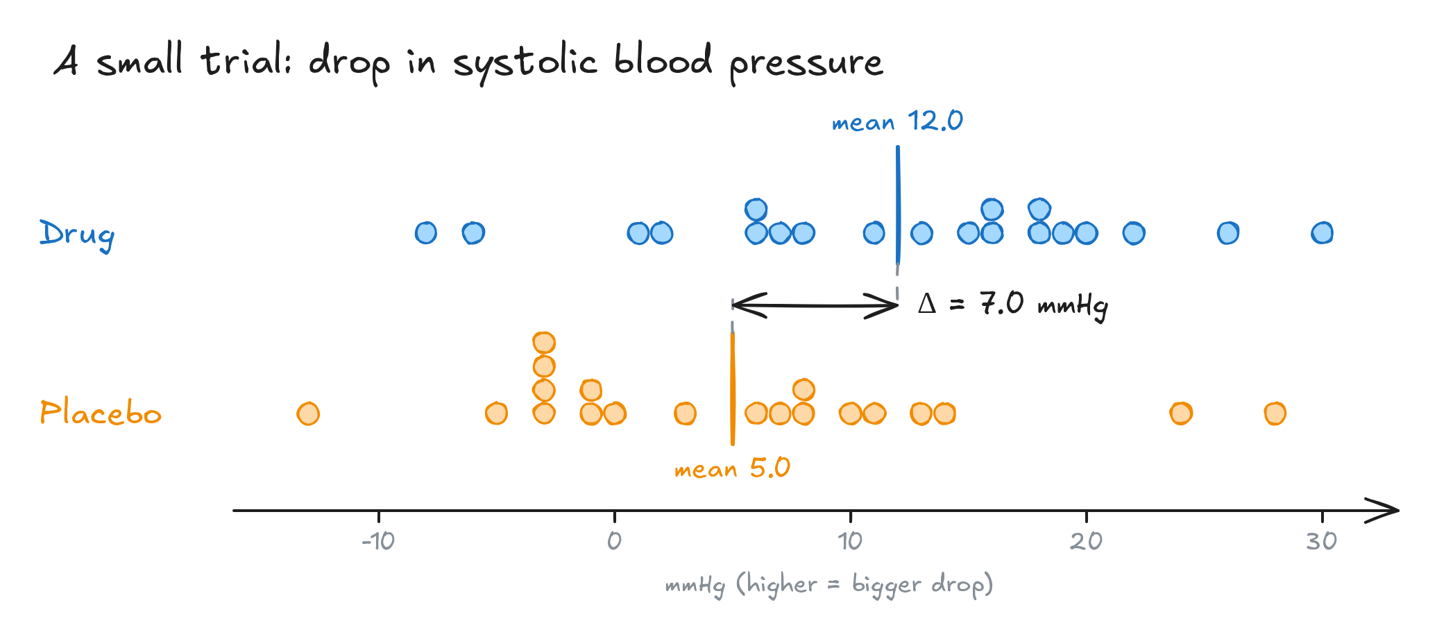
Fig. 1. Blood-pressure drop in each patient
The drug group dropped 12.0 mmHg on average and the placebo group 5.0 mmHg, a difference of 7 mmHg. But patients vary a lot (the standard deviation is about 10 mmHg in both groups). So does the drug work, or did we just get lucky?
2. Start by assuming nothing is going on
Statistics answers this question backwards. First we state a skeptical null hypothesis H₀, then we ask whether the data make it hard to believe:
\[H_0:\ \mu_{\text{drug}} = \mu_{\text{placebo}} \qquad\qquad H_1:\ \mu_{\text{drug}} \neq \mu_{\text{placebo}}\]It works like a courtroom: the drug is presumed useless until the evidence makes that implausible.
Even a useless drug would not produce two identical averages, because patients differ and blood pressure fluctuates from day to day. Chance alone creates differences. So the real question is:
If the drug did nothing, how often would chance alone produce a difference as big as 7 mmHg?
3. Build the “nothing is going on” world by shuffling
If the drug does nothing, the labels “drug” and “placebo” carry no information: each patient would have had the same blood-pressure drop either way. That means we can:
- pool all 40 measurements,
- deal them at random into two new groups of 20,
- compute the difference in means, Δ*,
- repeat 10,000 times.
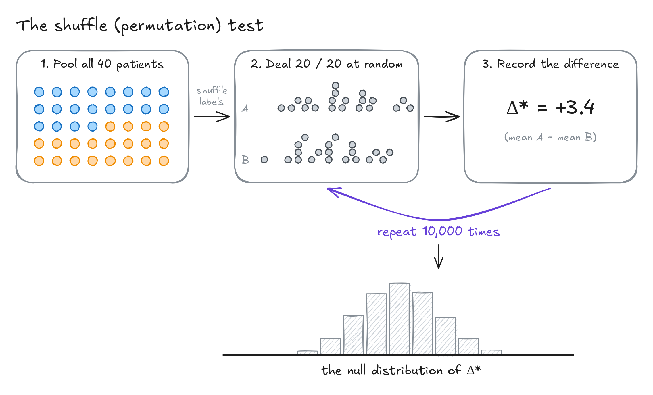
Fig. 2. The shuffle (permutation) test
The 10,000 shuffled differences form the null distribution: what differences look like when the labels are meaningless. Most land near 0, and big differences are rare.
4. The p-value
Now place the real result in that distribution. We count every shuffle at least as extreme as ours in either direction (Δ* ≥ 7 or Δ* ≤ −7). This is called a two-sided test. There were 157 + 179 = 336 such shuffles out of 10,000:
\[p \approx \frac{336}{10{,}000} = 0.034\]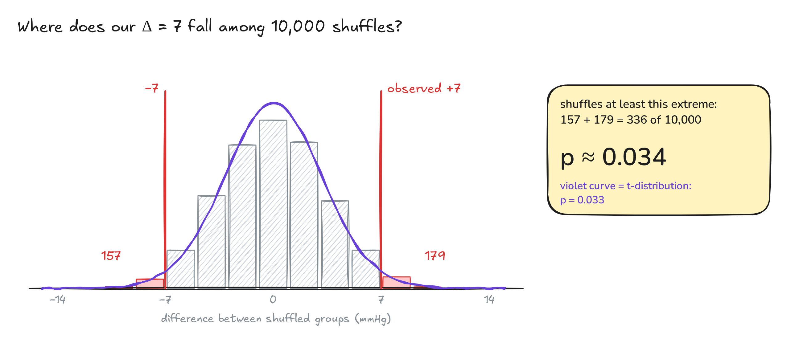
Fig. 3. The observed difference against the null distribution
That is the whole idea. p is the fraction of the “nothing is going on” world that looks at least as extreme as what we saw. A small p means our data would be surprising if H₀ were true.
Why count both tails? Before the study we did not know which direction the drug might act. A one-sided test counts only one tail and roughly halves p. It is only honest if the direction was fixed before looking at the data.
5. The shortcut: the two-sample t-test
Shuffling is intuitive, but when the data are roughly normal a formula gives almost the same answer instantly. It turns the difference into a signal-to-noise ratio:
\[t = \frac{\bar{x}_{\text{drug}} - \bar{x}_{\text{placebo}}}{s_p\sqrt{\frac{1}{n_1}+\frac{1}{n_2}}}, \qquad s_p = \sqrt{\frac{(n_1-1)s_1^2+(n_2-1)s_2^2}{n_1+n_2-2}}\]| Quantity | Formula | Our trial |
|---|---|---|
| Signal: difference in means | \(\bar{x}_1-\bar{x}_2\) | 12.0 − 5.0 = 7.0 mmHg |
| Pooled standard deviation | \(s_p\) | 10.0 mmHg |
| Noise: standard error | \(s_p\sqrt{1/n_1+1/n_2}\) | 10.0 × √0.1 = 3.16 mmHg |
| Test statistic | \(t\) = signal / noise | 7.0 / 3.16 = 2.21 |
| Degrees of freedom | \(n_1+n_2-2\) | 38 |
| Two-sided p-value | \(2\,\big(1-F_{t_{38}}(\lvert t\rvert)\big)\) | 0.033 |
If H₀ is true, t follows a t-distribution with 38 degrees of freedom. The p-value is the area in both tails beyond ±2.21 (the violet curve in Fig. 3), and it matches the shuffling answer almost exactly.
6. From p to a decision: α, errors and power
Before the study, choose a significance level α, conventionally 0.05. If p ≤ α, reject H₀ and call the result “statistically significant”. Our p = 0.033 qualifies. Any rule like this can be wrong in two ways:
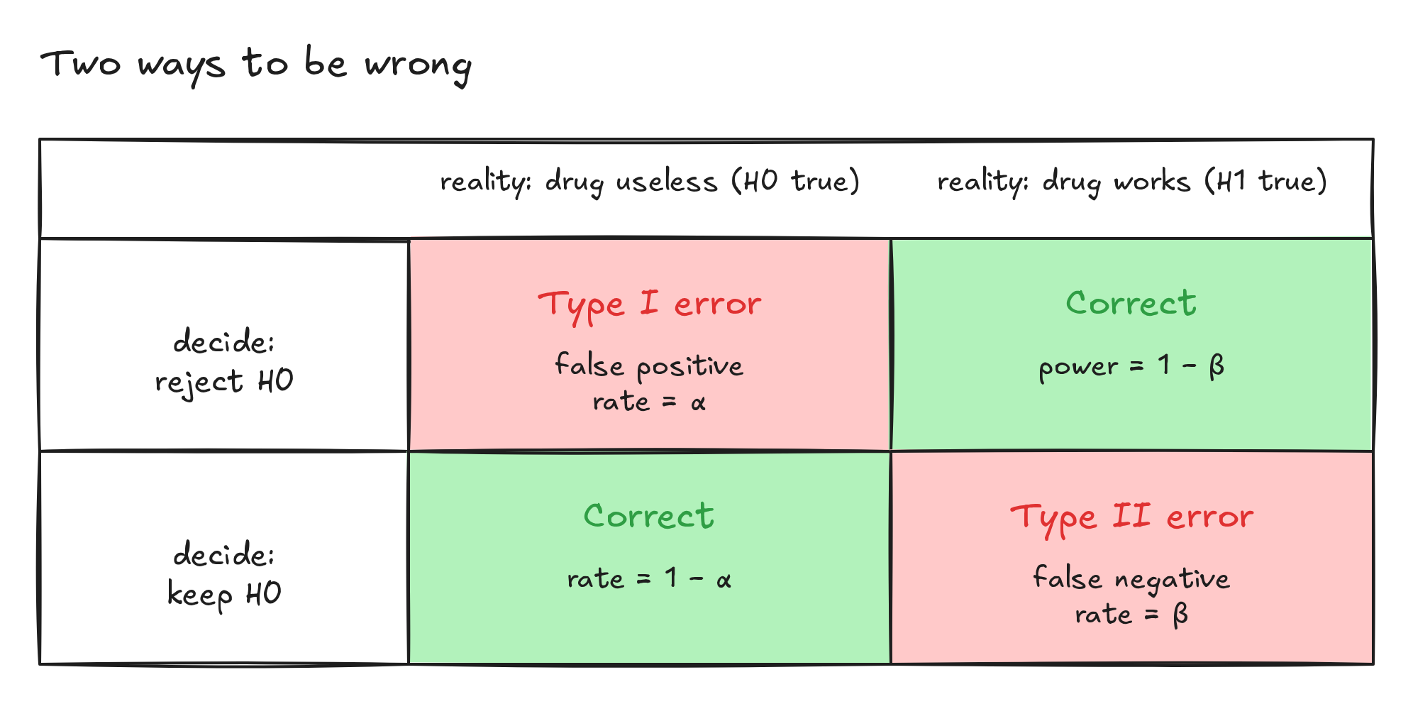
Fig. 4. Two ways to be wrong
- Type I error (false positive): rejecting H₀ when it is true. By construction this happens with probability α.
- Type II error (false negative): keeping H₀ when the drug actually works. Its probability is called β.
- Power = 1 − β: the chance of detecting an effect that is really there. Studies choose their sample size to reach high power, typically 80–90%.
7. What moves p, and why “significant” ≠ “important”
With equal group sizes n, the t statistic can be written as
\[t = \frac{\text{effect}}{\text{noise}\times\sqrt{2/n}}\]So p depends on three things at once: the size of the effect, the noise in the data, and the sample size.
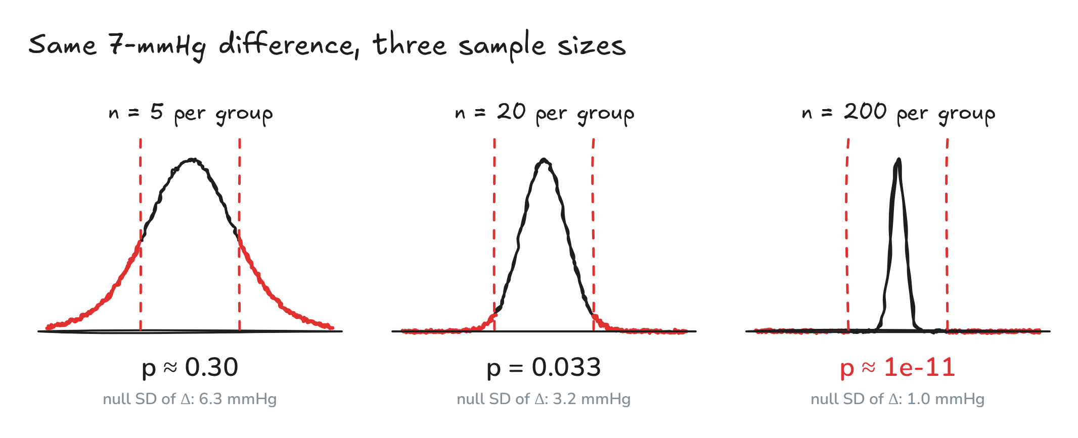
Fig. 5. The same 7-mmHg difference with three sample sizes
| Same 7-mmHg difference, SD 10 | n per group | t | p |
|---|---|---|---|
| Tiny pilot study | 5 | 1.11 | 0.30 |
| Our trial | 20 | 2.21 | 0.033 |
| Large trial | 200 | 7.00 | about 10⁻¹¹ |
The flip side: a clinically meaningless 0.5-mmHg effect becomes “significant” (p ≈ 0.04) with 3,500 patients per group. Statistical significance is not clinical importance.
That is why the effect size should always be reported with a confidence interval:
\[\bar{x}_1-\bar{x}_2 \;\pm\; t_{0.975,\,38}\times SE \;=\; 7.0 \pm 2.02\times 3.16 \;=\; [\,0.6,\ 13.4\,]\ \text{mmHg}\]The data are compatible with anything from a negligible 0.6-mmHg benefit to a large 13.4-mmHg one. The interval excludes 0, which carries the same information as p < 0.05, but it also shows how big the effect might be.
8. Four classic traps
-
“p = 0.033 means a 3.3% chance that H₀ is true.” No. The p-value is computed assuming H₀ is true, and P(data H₀) ≠ P(H₀ data). The probability of a hypothesis needs prior information (Bayes’ theorem). - “1 − p = 96.7% chance that the drug works.” The same mistake in reverse.
- “p > 0.05 proves there is no effect.” Absence of evidence is not evidence of absence. The study may simply be too small (low power), so look at the confidence interval.
- “A tiny p means a big effect.” p mixes effect size with sample size. Read the effect size and its CI.
Two more points are worth remembering. The 0.05 line is a convention, not a law of nature: p = 0.049 and p = 0.051 carry nearly the same evidence. And trying many analyses until one comes out “significant” (p-hacking) makes the p-value meaningless.
9. Many tests at once: genomics
| Suppose you test 20,000 genes for differential expression and none truly differ. When H₀ is true and the test is valid, p-values are uniformly distributed between 0 and 1, so P(p ≤ α | H₀) = α. About |
genes will look “significant” by chance alone (983 in our simulation).
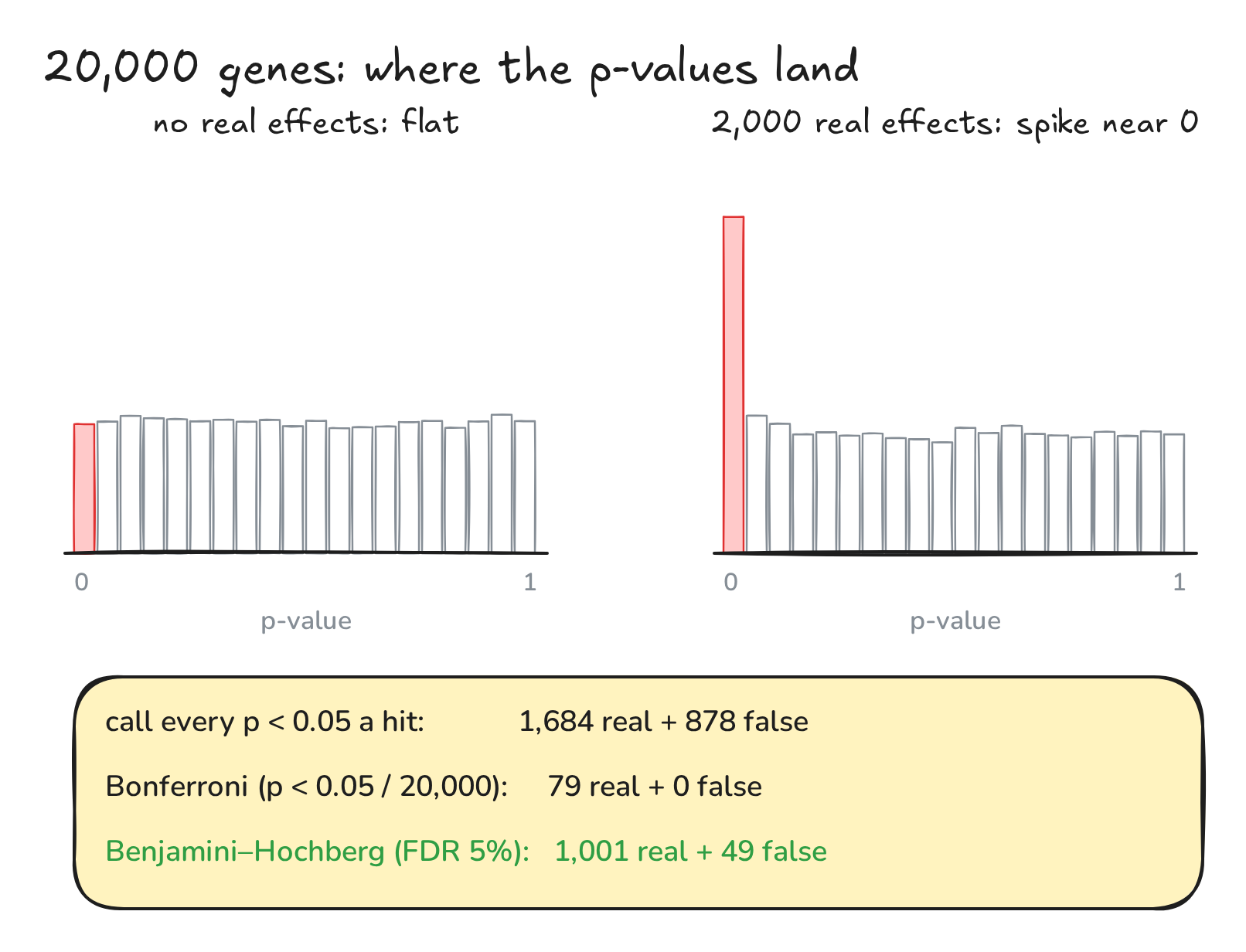
Fig. 6. p-value histograms and the effect of multiple-testing correction
The right panel of Fig. 6 adds 2,000 genes with real effects. They show up as a spike near 0 on top of the flat background. Two standard corrections:
- Bonferroni controls the chance of making any false positive (the family-wise error rate). It tests each gene at α/m = 0.05 / 20,000 = 2.5 × 10⁻⁶. That is very safe, but in the simulation it found only 79 of the 2,000 real effects.
- Benjamini–Hochberg controls the false discovery rate (FDR): the expected share of false hits among your discoveries.
- Sort the p-values from smallest to largest: \(p_{(1)} \le \dots \le p_{(m)}\).
- Find the largest k with \(p_{(k)} \le \frac{k}{m}\,q\).
- Call the k smallest p-values significant.
At q = 0.05 it found 1,001 real effects and 49 false ones (4.7%), exactly what it promises. This is the adjusted p-value that DESeq2 (
padj), edgeR (FDR) and limma (adj.P.Val) report.
10. Cheat sheet
| Term | Meaning |
|---|---|
| Null hypothesis H₀ | “Nothing is going on”: no difference, no effect |
| Test statistic | One number summarizing the evidence, e.g. t = signal / noise |
| Null distribution | How the statistic behaves when H₀ is true |
| p-value | P(result at least as extreme as observed | H₀ true) |
| α (significance level) | Threshold fixed in advance; equals the Type I error rate |
| Type I / Type II error | False positive / false negative |
| Power (1 − β) | Probability of detecting a real effect |
| Effect size + 95% CI | How big the effect is, and how precisely we know it |
| FDR (BH-adjusted p) | Expected share of false positives among discoveries |
Try it yourself (Python)
import numpy as np
from scipy import stats

drug    = np.array([22, 20, 13, 19, 6, -6, 30, 18, -8, 2, 7, 16, 26, 16, 8, 18, 11, 15, 6, 1])
placebo = np.array([14, -1, 3, -3, -3, -1, 8, 13, 7, -3, 28, 10, 11, -3, 0, 8, -13, -5, 6, 24])

# 1) two-sample t-test (equal variances, two-sided)
t, p = stats.ttest_ind(drug, placebo)
print(f"t = {t:.2f}, p = {p:.4f}")   # t = 2.21, p = 0.0331

# 2) permutation (shuffle) test with 10,000 shuffles
rng = np.random.default_rng(1013)
pooled = np.concatenate([drug, placebo])
obs = drug.mean() - placebo.mean()
diffs = np.empty(10_000)
for i in range(10_000):
    perm = rng.permutation(40)
    diffs[i] = pooled[perm[:20]].mean() - pooled[perm[20:]].mean()
print(f"permutation p = {np.mean(np.abs(diffs) >= abs(obs) - 1e-9):.4f}")   # permutation p = 0.0336

# 3) 95% confidence interval for the difference in means
sp = np.sqrt((19 * drug.var(ddof=1) + 19 * placebo.var(ddof=1)) / 38)
se = sp * np.sqrt(1 / 20 + 1 / 20)
tcrit = stats.t.ppf(0.975, df=38)
print(f"95% CI: [{obs - tcrit * se:.1f}, {obs + tcrit * se:.1f}] mmHg")   # 95% CI: [0.6, 13.4] mmHg
Figures were drawn with Excalidraw; the editable sources open directly on excalidraw.com: Fig. 1, Fig. 2, Fig. 3, Fig. 4, Fig. 5, Fig. 6. The video was animated with Remotion and narrated with a synthetic (text-to-speech) voice. Music: “Deliberate Thought” by Kevin MacLeod (incompetech.com), licensed under CC BY 4.0.