In one sentence: a variational autoencoder learns a smooth, probabilistic map of your data, turning discrete molecules, cells and proteins into a space you can measure, interpolate and optimize.
It is not an oracle, and it is not the only generator, but it makes biology navigable.
The video above (4:11) tells the story. This page keeps the same order and adds what I measured. Both models were trained from scratch on public data, and every number below is measured, not quoted, unless it carries a citation.
1. The problem is the size of the room
There are roughly \(10^{60}\) drug-like molecules (a common estimate). Chemists have made on the order of \(10^{8}\). Bringing one drug to approval costs about $2.6 billion (DiMasi et al., 2016), and around nine in ten clinical candidates fail. You cannot enumerate this space, so you need a way to move through it.
The obstacle is that chemistry and biology are written in discrete symbols. A molecule is a string; a cell is a vector of integer counts. You cannot take a derivative of a string.
Measured: a one-character edit is not a small step. I made every single-character substitution of aspirin’s SMILES over a small alphabet, 168 edits in total. 87% stopped being a molecule at all. Of those that still parsed, the mean Tanimoto similarity to aspirin was only 0.57. An edit either breaks the string or silently hands you a different compound. Neither is a gradient.
2. The one idea: a cloud, not a dot
An autoencoder squeezes an input through a narrow code \(z\) and rebuilds it. A plain autoencoder pins each input to a point, and the space between points is undefined: sample there and the decoder returns noise.
A VAE maps each input to a small cloud instead:
\[q_\phi(z\mid x)=\mathcal{N}\big(\mu_\phi(x),\,\sigma_\phi^2(x)\big)\]Sampling stays differentiable through the reparameterisation trick, which moves the randomness into an external \(\varepsilon\) so gradients still reach \(\mu\) and \(\sigma\):
\[z=\mu+\sigma\odot\varepsilon,\qquad \varepsilon\sim\mathcal{N}(0,\mathbf{I})\]The training objective has two terms that pull against each other:
\[\mathcal{L}\;=\;\underbrace{-\log p_\theta(x\mid z)}_{\text{reconstruct}}\;+\;\beta\,\underbrace{D_{\mathrm{KL}}\big(q_\phi(z\mid x)\,\|\,\mathcal{N}(0,\mathbf{I})\big)}_{\text{organize}}\]Reconstruction wants a sharp code that stores every detail. The KL term pulls every cloud toward one shared region, so clouds overlap and fill the space with no holes. That tension is the model: the code keeps what is needed to rebuild the data and discards the rest.
3. Build one: 2,638 immune cells
I trained a scVI-style VAE on the public 10x Genomics PBMC3k dataset: 2,638 cells, 2,000 highly variable genes, a 10-dimensional latent space, 91.1% zeros in the count matrix, about 1.1 M parameters, 1.5 minutes on two CPU cores. The decoder outputs the parameters of a negative binomial, and expected counts are the cell’s library size times a softmax over genes, so noise and sequencing depth are handled explicitly and \(z\) is free to carry cell state.
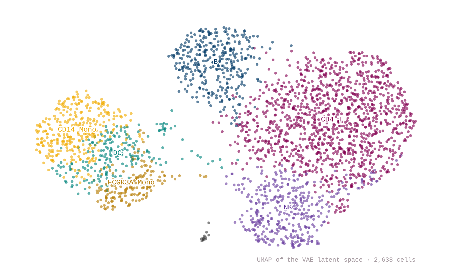
Fig. 1. UMAP of the VAE latent space. Nothing was told what a B cell is: clusters were found on the latent and then named by canonical markers.
Walking between two cell states. Take the CD4 T centroid and the CD14 monocyte centroid, walk the straight line between them in latent space, and decode every step:
\[z(t)=(1-t)\,z_A+t\,z_B\]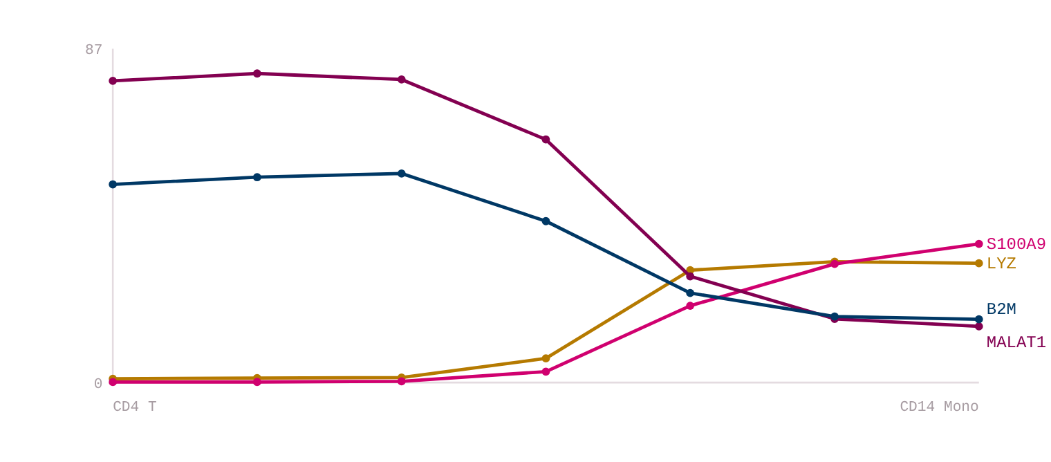
Fig. 2. Decoded expression at a fixed library size. LYZ rises 1.0 → 31.3 and S100A9 0.14 → 36.4; MALAT1 (79.1 → 14.7) and B2M (51.9 → 16.6) fall away. The two rising genes are canonical myeloid markers; the falling two were picked by the data as the genes that changed most.
What the noise model buys. Dropout is the defining nuisance of single-cell data: a gene is expressed but the experiment sees zero. Because the decoder predicts an expected count from the whole cell, it fills these in.
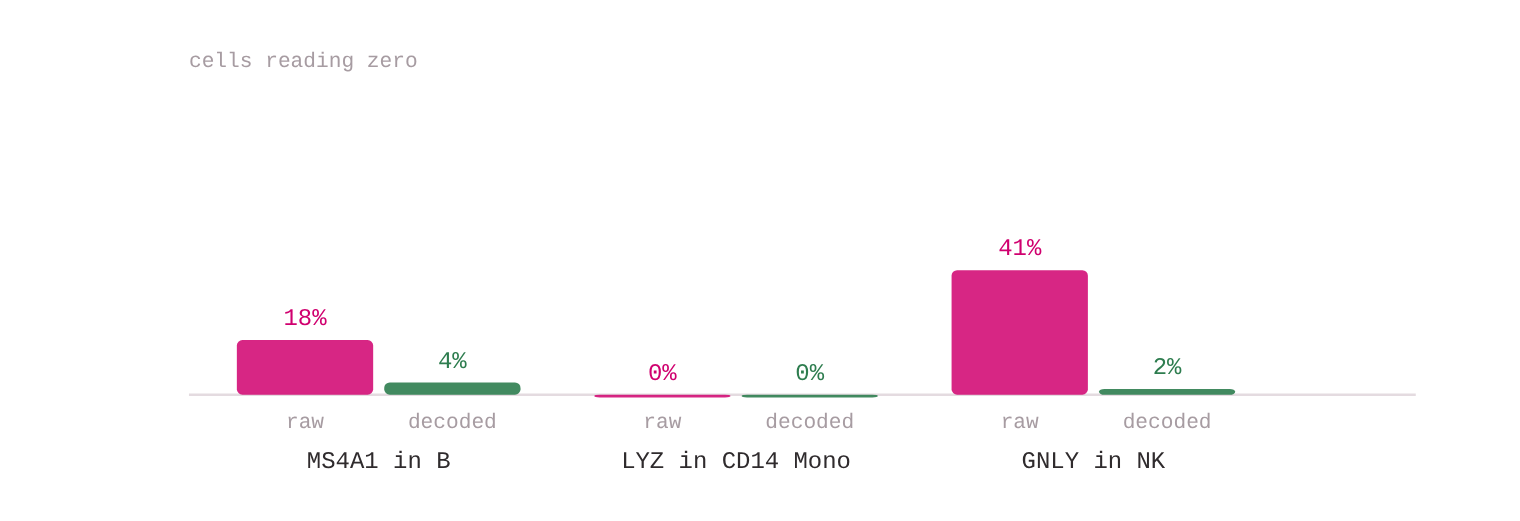
Fig. 3. 41% of NK cells read zero GNLY in the raw counts; after decoding, 2% do. This is not blanket smoothing: the GNLY mean in non-NK cells moves only 0.14 → 0.17.
4. Build two: 240,000 molecules
The second model encodes ZINC-250k molecules as SELFIES tokens (56-dimensional latent space, about 1.1 M parameters) with a small head that predicts drug-likeness (QED) and logP from \(z\). That head does the organising: a ridge probe recovers QED from the latent mean at \(R^2=0.71\) and logP at \(0.96\), while the first two principal components hold only 15% of the variance. So the map is drawn on the model’s own property directions, not on PCA.
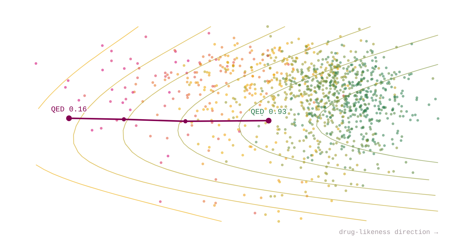
Fig. 4. 1,600 molecules coloured by drug-likeness, with iso-QED contours. The line is gradient ascent on the property head, run in latent space.
Starting from a latent point that decodes to QED 0.16 and ascending the model’s own prediction while decoding as we go:

Fig. 5. Decoded molecules at steps 0, 5, 10 and 20. True QED, measured with RDKit rather than predicted, goes 0.16 → 0.93.
5. What I would tell a colleague
The VAE is no longer the strongest generator: diffusion and sequence models draw better molecules. What endures is the other half, a smooth low-dimensional space with an explicit noise model and calibrated uncertainty. That is why scVI, scGen, CPA and totalVI remain a backbone of single-cell modelling. scGen and CPA do arithmetic in the latent space to predict responses to unseen drugs and doses:
\[z_{\text{pred}}=z_{\text{control}}+\delta_{\text{drug}}\]Others score tens of millions of protein variants for disease risk (EVE) or model T-cell receptor repertoires (Davidsen et al., 2019).
Honest limits of what you just saw:
- My cell latent is worse than PCA at separating cell types. Silhouette 0.105 against 0.383 for a 10-component PCA on the same genes. On one clean batch PCA is a strong baseline; a VAE earns its keep with batches to absorb, or when you want the generative half: denoising, counterfactuals, uncertainty.
- 100% validity proves almost nothing. SELFIES is built so every string decodes to a molecule, so validity measures the representation, not the model’s chemistry. The original SMILES chemical VAE reached about 74% valid prior samples.
- The molecule model barely reconstructs. Exact-match reconstruction was 0.1%, after about one epoch of training. The code captures properties, not identity, so treat the interpolation as a tour of the property landscape, not faithful editing of one compound.
- The property head over-promises. Along the climb, its predicted QED sat a mean 0.16 away from the measured value, so any latent optimizer needs an external scorer in the loop.
A valid molecule is not a viable drug, and a predicted cell state is not an experiment. AI narrows the funnel; it does not skip the assays, the toxicology or the trials. Rentosertib, an AI-found target with an AI-designed molecule, needed a phase 2a readout in 2025 (60 mg once daily: +98.4 mL FVC versus −20.3 mL on placebo, 71 patients) before it meant anything.
6. The core, in a few lines
mu, logvar = encoder(torch.log1p(x))                       # counts in, distribution out
z   = mu + torch.exp(0.5 * logvar) * torch.randn_like(mu)  # reparameterisation
rho = torch.softmax(decoder(z), -1)                        # per-gene share of the library
mu_gene = x.sum(1, keepdim=True) * rho                     # expected counts

rec  = nb_nll(x, mu_gene, theta)                           # negative binomial, not MSE
kl   = 0.5 * (mu**2 + logvar.exp() - 1 - logvar).sum(1)
loss = (rec + beta * kl).mean()                            # beta warmed up from 0
Two details carry most of the weight: the likelihood is a negative binomial over raw counts, so overdispersion and dropout are modelled instead of smoothed away; and library size multiplies the decoder output rather than entering the encoder, so depth never has to be encoded in \(z\).
Sources
- Kingma & Welling, Auto-Encoding Variational Bayes, ICLR 2014. arXiv:1312.6114
- Lopez et al., scVI, Nature Methods 2018. doi:10.1038/s41592-018-0229-2
- Lotfollahi et al., scGen, Nature Methods 2019. doi:10.1038/s41592-019-0494-8
- Lotfollahi et al., CPA, Mol Syst Biol 2023. doi:10.15252/msb.202211517
- Gómez-Bombarelli et al., chemical VAE, ACS Cent Sci 2018. arXiv:1610.02415
- Jin, Barzilay & Jaakkola, JT-VAE, ICML 2018. arXiv:1802.04364
- Frazer et al., EVE, Nature 2021.
- Davidsen et al., TCR generative models, eLife 2019. doi:10.7554/eLife.46935
- Zhavoronkov et al., DDR1 inhibitors, Nat Biotechnol 2019. doi:10.1038/s41587-019-0224-x
- Xu et al., rentosertib, Nature Medicine 2025. doi:10.1038/s41591-025-03743-2
- DiMasi, Grabowski & Hansen, J Health Econ 2016; Sun et al., Acta Pharm Sin B 2022; Bohacek et al. 1996.
- Data: 10x Genomics PBMC3k (public); ZINC-250k drug-like subset.
Both models were trained in a sandbox from scratch; the cell and molecule figures are drawn from the exported results of those runs. Animated with Remotion and narrated with a synthetic (text-to-speech) voice. Music: “Deliberate Thought” by Kevin MacLeod (incompetech.com), licensed CC BY 4.0. Created by Miao Li.